Съдържание

GeCAA 2020, Отборен тур, „Спектрални изкривявания на реликтовото лъчение“ — Задача 1. Spectral Distortions of the CMB

Оригинал на условието (PDF)Съобщи за грешка

Всички материали от GeCAA 2020

Spectral Distortions of the CMB — Team Exam

Условие

In this problem, you will investigate whether a proposed satellite mission, the Primordial Inflation Experiment (PIXIE, Kogut et al., 2011, 2016), will be able to detect spectral distortions of the Cosmic Microwave Background (CMB).

Over the past 30 years, the CMB has provided research opportunities for precision cosmology $^{1}$ , the results of which have solidified our understanding of the history of our universe. The spatial anisotropies of the CMB have been at the forefront of both experiment and theory, and have driven the field forward. As per our understanding, these spatial anisotropies can reveal details about the size and physical properties of the primordial fluctuations in matter distribution leading to the rise of the structure that we see today. The interaction of matter with photons, on the other hand should lead to spectral anisotropies. Such anisotropies have been theoretically predicted, but have never been detected so far.

In 1992, the FIRAS instrument on NASA’s Cosmic Background Explorer (COBE) (Fixsen et al., 1996; Mather et al., 1994; Fixsen, 2009) mission showed that the CMB spectrum is a near-perfect blackbody, isotropic to the level of one part in $10^5$ , with temperature $T_{\mathrm{CMB}} = (2.725 \pm 0.001)\,\mathrm{K}$ .

Radiation is thermalized at very high redshifts (well before and up until the decoupling of radiation and matter) due to a number of radiative processes, such as Compton, inverse Compton, double Compton scattering and bremsstrahlung, each one dominating at different energy regimes (and thus redshifts). $^{2}$

Physical processes such as reionization and structure formation, decaying or annihilating particles, dissipation of primordial density fluctuations, adiabatic cooling of matter and recombination, as well as cosmic strings, primordial black holes, small-scale magnetic fields, can lead to distortions to the blackbody shape of the spectrum of CMB (Chluba, 2014; Chluba and Jeong, 2014; Hill et al., 2015; Tashiro, 2014).

Spectral distortions of the CMB, if present, were not detectable at the precision level of the FIRAS instrument. PIXIE will provide a sensitivity improved by 76 times compared to its similar predecessor.

As the Universe expands, processes responsible for maintaining thermalization become less effective. This then allows spectral distortions to be developed. The distortions created between redshift $z \approx 10^6$ (when double Compton scattering decouples) and $z \approx 10^5$ (when Compton scattering no longer contributes to thermalization) are characterized by a chemical potential $^{3}$ and are called " $\mu$ distortions" (Zeldovich and Sunyaev, 1969; Sunyaev and Zeldovich, 1970; Illarionov and Siuniaev, 1975; Sunyaev and Khatri, 2013). At redshifts below $1.5 \times 10^4$ , after thermalization decoupling, Compton and inverse Compton scattering produce the so-called " $y$ distortions" $^{4}$ (Zeldovich and Sunyaev, 1969; Sunyaev and Zeldovich, 1972). For $1.5 \times 10^4 < z < 2 \times 10^5$ , we get a distortion spectrum that is intermediate between those of $y$ and $\mu$ -type distortions (Khatri and Sunyaev, 2012).

The two different types of distortions have different frequency dependence and this can suggest the type (as well as redshift) of interactions that give rise to spectral distortions.

Assume PIXIE will have the sensitivity as described in Table 1.

$^{1}$ The branch of cosmology that makes detailed quantitative predictions and measurements of properties of the Universe

$^{2}$ You can read more at https://ned.ipac.caltech.edu/level5/Sept05/Gawiser2/Gawiser1.html

$^{3}$ The chemical potential $\mu$ is a quantity that expresses energy that is absorbed or released when the number of particles -in this case, photons- in a system changes. Here, it is measured in units of $kT$ and is thus dimensionless.

$^{4}y$ is a parameter that expresses by how much a photon will change its energy due to repeated scatterings in a medium of finite extend.

Frequency [GHz]	14.4	374.6	734.9	1095.1
PIXIE Sensitivity [Jy/sr]	3.6035	3.7700	4.2859	5.1598

Table 1: PIXIE Sensitivity (Jy refers to the unit Jansky)

Spectral Distortions Modeling

y distortion PIXIE can shed light on the history of star formation by looking at the spectral distortions produced during the epoch of reionization. The CMB photons undergo inverse Compton scattering off the gas that has been ionized by early stars. These distortions are parametrized by $y$ which expresses the mean number of scatterings times the average energy change that a photon suffers in a scattering. The respective intensity contribution is given by:

\Delta I_{\nu,y} = I_0 \frac{x^4 e^x}{(e^x - 1)^2}\left[x \coth\left(\frac{x}{2}\right) - 4\right] y, \qquad (1)

where $I_0 = \frac{2h}{c^2}(\frac{kT_0}{h})^3 = 270\,\mathrm{MJy/sr}$ for $T_0 = 2.726\,\mathrm{K}$ , and $x = \frac{h\nu}{kT_0}$ . We take $y = 1.7 \times 10^{-6}$ for our fiducial value (assumed value for comparison).

$\mu$ distortion The amplitude of density fluctuations during inflation translates into energy injection in the CMB for redshifts $10^5 < z < 10^6$ which leads to $\mu$ distortions characterized by the chemical potential, with intensity given by

\Delta I_{\nu,\mu} = I_0 \frac{x^4 e^x}{(e^x - 1)^2}\left[\frac{1}{\beta} - \frac{1}{x}\right] \mu, \qquad (2)

where $I_0 = \frac{2h}{c^2}(\frac{kT_0}{h})^3 = 270\,\mathrm{MJy/sr}$ for $T_0 = 2.726\,\mathrm{K}$ , $x = \frac{h\nu}{kT_0}$ and $\beta = 2.1923$ .

A suitable fiducial value for $\mu$ is $\mu = 2 \times 10^{-8}$ (Abitbol et al., 2017).

Your task, as a team, is to calculate the expected standard deviations of the $y$ and $\mu$ parameters, if PIXIE were to try to measure them in the bands given in Table 1. This will tell us if the $y$ and $\mu$ distortions will be detectable, assuming the fiducial values given above.

In order to calculate that, you can use the matrix $^{5}$ :

F_{ij} = \sum_{a,b} \left(\frac{\partial(\Delta I_\nu)}{\partial p_i}\right)_a C^{-1}_{ab} \left(\frac{\partial(\Delta I_\nu)}{\partial p_j}\right)_b \qquad (3)

called the Fisher Information Matrix (see for example Verde, 2010). $a, b$ are indexing frequency, and $p_i, p_j$ are parameters of the model (in our case, the two free parameters for the spectral distortions, $y$ and $\mu$ , all other parameters assumed fixed). $C^{-1}_{ab}$ is the inverse of the covariance matrix of the experiment. Inverting the $F_{ij}$ matrix and taking the square root of the diagonal gives us the standard deviations expected for each parameter.

$^{5}$ For students not familiar with matrix notation and/or partial derivatives, a basic introduction for these can be found in any good introductory textbook on calculus / analysis

(a) Make a plot of $\Delta I_{\nu,y}$ and $\Delta I_{\nu,\mu}$ over the range of frequencies 14.4GHz to 1100.1 GHz, assuming the fiducial values for $y$ and $\mu$ . [18 т.]

(b) Calculate the analytical forms of $\frac{\partial \Delta I_{\nu,\mu}}{\partial \mu}$ and $\frac{\partial \Delta I_{\nu,y}}{\partial y}$ .
Then, evaluate them at the 4 frequencies given in Table 1. [10 т.]

(c) Calculate the covariance matrix $C_{ab}$ for PIXIE sensitivity in frequency bands using Table 1. The covariance matrix has the variance (square of the sensitivity) of the frequency bands on the diagonal, and the covariance of the bands on the other entries. In this problem, assume the frequency bands are uncorrelated and their covariance is thus 0. [8 т.]

(d) Calculate the inverse $C^{-1}_{ab}$ of the PIXIE covariance matrix. [4 т.]

(e) Assuming PIXIE is trying to model only the $y$ and $\mu$ distortions, and ignoring other foregrounds, calculate the Fisher Information Matrix, and the standard deviations for the parameters $y$ and $\mu$ .

(i) Would the $y$ distortion be detectable with PIXIE?

(ii) Would the $\mu$ distortion be detectable with PIXIE?

For the distortion to be detectable, the standard deviation on the parameter should be less than the value of the parameter. [20 т.]

Notes:

Useful Constants and Units
- $h = 6.626\,070\,04 \times 10^{-34}\,\mathrm{J\,s}$
- $k = 1.380\,648\,52 \times 10^{-23}\,\mathrm{J\,K^{-1}}$
- $1\,\mathrm{Jy} = 10^{-26}\,\mathrm{W/m^2/Hz}$
In this analysis, for each given frequency, the only free parameters of the functions $\Delta I_{\nu,y}$ and $\Delta I_{\nu,\mu}$ are $y$ and $\mu$ respectively.
A partial derivative $\frac{\partial f}{\partial x}$ of a multi-variable function $f(x, y, z, ...)$ with respect to a single variable $x$ is the process of calculating derivative with respect to the said variable $x$ , while all the other variables are kept constant.
In reality, PIXIE will have to model other foregrounds as well, such as the foregrounds coming from the synchrotron emission in the galaxy, the thermal radiation from the dust present in the interstellar medium, the free-free emission, cosmic infrared background etc. But we will ignore these contributions for the purpose of the problem.

References

M. H. Abitbol, J. Chluba, J. C. Hill, and B. R. Johnson. Prospects for measuring cosmic microwave background spectral distortions in the presence of foregrounds. Monthly Notices of the Royal Astronomical Society, Volume 471, Issue 1, p.1126-1140, 471:1126–1140, oct 2017. doi: 10.1093/mnras/stx1653. URL https://ui.adsabs.harvard.edu/abs/2017MNRAS.471.1126A.

J. Chluba. Science with CMB spectral distortions, may 2014. URL https://ui.adsabs.harvard.edu/abs/2014arXiv1405.6938C.

J. Chluba and D. Jeong. Teasing bits of information out of the CMB energy spectrum. Monthly Notices of the Royal Astronomical Society, Volume 438, Issue 3, p.2065-2082, 438:2065–2082, mar 2014. doi: 10.1093/mnras/stt2327. URL https://ui.adsabs.harvard.edu/abs/2014MNRAS.438.2065C.

D. J. Fixsen. The Temperature of the Cosmic Microwave Background. The Astrophysical Journal, Volume 707, Issue 2, pp. 916-920 (2009)., 707:916–920, dec 2009. doi: 10.1088/0004-637X/707/2/916. URL https://ui.adsabs.harvard.edu/abs/2009ApJ...707..916F.

D. J. Fixsen, E. S. Cheng, J. M. Gales, J. C. Mather, R. A. Shafer, and E. L. Wright. The Cosmic Microwave Background Spectrum from the Full COBE FIRAS Data Set. Astrophysical Journal v.473, p.576, 473:576, dec 1996. doi: 10.1086/178173. URL https://ui.adsabs.harvard.edu/abs/1996ApJ...473..576F.

J. C. Hill, N. Battaglia, J. Chluba, S. Ferraro, E. Schaan, and D. N. Spergel. Taking the Universe’s Temperature with Spectral Distortions of the Cosmic Microwave Background. Physical Review Letters, Volume 115, Issue 26, id.261301, 115:261301, dec 2015. doi: 10.1103/PhysRevLett.115.261301. URL https://ui.adsabs.harvard.edu/abs/2015PhRvL.115z1301H.

A. F. Illarionov and R. A. Siuniaev. Comptonization, characteristic radiation spectra, and thermal balance of low-density plasma. Soviet Astronomy, vol. 18, Jan.-Feb. 1975, p. 413-419. Translation., 18:413–419, feb 1975. URL https://ui.adsabs.harvard.edu/abs/1975SvA....18..413I.

R. Khatri and R. A. Sunyaev. Beyond y and $\mu$ : the shape of the CMB spectral distortions in the intermediate epoch, 1.5 Ã 104lesssimzlesssim2 Ã 105. Journal of Cosmology and Astroparticle Physics, Issue 09, article id. 016 (2012)., 2012:16, sep 2012. doi: 10.1088/1475-7516/2012/09/016. URL https://ui.adsabs.harvard.edu/abs/2012JCAP...09..016K.

A. Kogut, D. J. Fixsen, D. T. Chuss, J. Dotson, E. Dwek, M. Halpern, G. F. Hinshaw, S. M. Meyer, S. H. Moseley, M. D. Seiffert, D. N. Spergel, and E. J. Wollack. The Primordial Inflation Explorer (PIXIE): a nulling polarimeter for cosmic microwave background observations. Journal of Cosmology and Astroparticle Physics, Issue 07, id. 025 (2011)., 2011:25, jul 2011. doi: 10.1088/1475-7516/2011/07/025. URL https://ui.adsabs.harvard.edu/abs/2011JCAP...07..025K.

A. Kogut, J. Chluba, D. J. Fixsen, S. Meyer, and D. Spergel. The Primordial Inflation Explorer (PIXIE). In Proceedings of the SPIE, Volume 9904, id. 99040W 23 pp. (2016)., volume 9904, page 99040W, jul 2016. doi: 10.1117/12.2231090. URL https://ui.adsabs.harvard.edu/abs/2016SPIE.9904E..0WK.

J. C. Mather, E. S. Cheng, D. A. Cottingham, R. E. Eplee Jr., D. J. Fixsen, T. Hewagama, R. B. Isaacman, K. A. Jensen, S. S. Meyer, P. D. Noerdlinger, S. M. Read, L. P. Rosen, R. A. Shafer, E. L. Wright, C. L. Bennett, N. W. Boggess, M. G. Hauser, T. Kelsall, S. H. Moseley Jr., R. F. Silverberg, G. F. Smoot, R. Weiss, and D. T. Wilkinson. Measurement of the Cosmic Microwave Background Spectrum by the COBE FIRAS Instrument. Astrophysical Journal v.420, p.439, 420:439, jan 1994. ISSN 0004-637X. doi: 10.1086/173574. URL https://ui.adsabs.harvard.edu/abs/1994ApJ...420..439M.

R. A. Sunyaev and R. Khatri. Unavoidable CMB Spectral Features and Blackbody Photosphere of Our Universe. International Journal of Modern Physics D, Volume 22, Issue 7, id. 1330014, 22:1330014, jun 2013. doi: 10.1142/S0218271813300140. URL https://ui.adsabs.harvard.edu/abs/2013IJMPD..2230014S.

R. A. Sunyaev and Y. B. Zeldovich. The interaction of matter and radiation in the hot model of the Universe, II. Astrophysics and Space Science, 7:20–30, apr 1970. ISSN 0004-640X. doi: 10.1007/BF00653472. URL $\texttt{https://ui.adsabs.harvard.edu/abs/1970Ap\{\&\}SS...7...20S}$ .

R. A. Sunyaev and Y. B. Zeldovich. Formation of Clusters of Galaxies; Protocluster Fragmentation and Intergalactic Gas Heating. Astronomy and Astrophysics, 20:189, aug 1972. ISSN 0004-6361. URL $\texttt{https://ui.adsabs.harvard.edu/abs/1972A\{\&\}A....20..189S}$ .

H. Tashiro. CMB spectral distortions and energy release in the early universe. Progress of Theoretical and Experimental Physics, Volume 2014, Issue 6, id.06B10727 pp., 2014:06B107, jun 2014. doi: 10.1093/ptep/ptu066. URL https://ui.adsabs.harvard.edu/abs/2014PTEP.2014fB107T.

L. Verde. Statistical Methods in Cosmology. In Lectures on Cosmology Accelerated Expansion of the Universe by Georg Wolschin, Lecture Notes in Physics vol. 800, Springer Berlin / Heidelberg, ISSN 1616-6361; ISBN 978-3-642-10597-5, pp.147-177, volume 800, pages 147–177. mar 2010. ISBN 1616-6361. doi: 10.1007/978-3-642-10598-2_4. URL https://ui.adsabs.harvard.edu/abs/2010LNP...800..147V.

Y. B. Zeldovich and R. A. Sunyaev. The Interaction of Matter and Radiation in a Hot-Model Universe. Astrophysics and Space Science, 4:301–316, jul 1969. ISSN 0004-640X. doi: 10.1007/BF00661821. URL $\texttt{https://ui.adsabs.harvard.edu/abs/1969Ap\{\&\}SS...4..301Z}$ .

Отговори

Решение

(a)

Solution

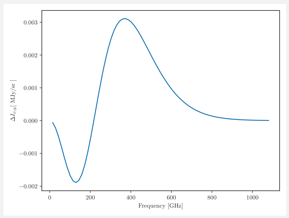
Plot of the y-distortion intensity ΔI_ν,y [MJy/sr] against Frequency [GHz] from about 14 to 1100 GHz: the curve starts near 0, dips to about −0.0019 near 130 GHz, crosses zero near 217 GHz, peaks at about 0.0031 near 370 GHz and decays to 0 by about 1000 GHz. Axis ticks 0–1000 GHz and −0.002 to 0.003. — $y$ distortion

correct $y$ plot function shape, consists of

correct scaling of the plot 2

correct maximum and minimum values of the functions, (=2x0.5) 1

correct 0 crossing of the function $\Delta I_{\nu,y}$ . Its positive numerical/graphical solution is $x \approx 3.83$ , which corresponds to a frequency of 217.5GHz. Students can find the 0 crossings graphically, but it needs to be within 30GHz of the correct answer of 217.5GHz to can be given full marks. Note: To find the 0 crossing for $\Delta I_{\nu,y}$ numerically, one needs to solve the transcendental Eq. $x\coth\left(\frac{x}{2}\right) = 4$ , which can also be written in the form $\exp(x) = \frac{4+x}{4-x}$ . The calculations method (ex: Newton’s method) might involve derivatives with respect to $x$ , so you might see lengthy calculations. 2

correct behaviour of the function at the lowest end of the frequency range 0.5

correct behaviour of the function at the highest end of the frequency range 0.5

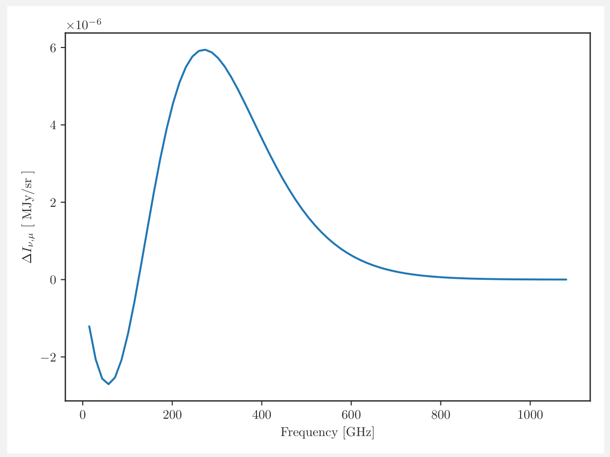
Plot of the μ-distortion intensity ΔI_ν,μ [MJy/sr] (scale ×10⁻⁶) against Frequency [GHz]: the curve starts at about −1.2, dips to about −2.7 near 60 GHz, crosses zero near 124 GHz, peaks at about 5.9 near 270 GHz and decays to 0 by about 900 GHz. Axis ticks 0–1000 GHz and −2 to 6. — $\mu$ distortion

correct $\mu$ plot function shape consists of

correct scaling of the plot 2

correct maximum and minimum values of the functions, (=2x0.5) 1

correct 0 crossing of the function $\Delta I_{\nu,\mu}$ . Its 0 crossing occurs at $x = \beta$ , which corresponds to a frequency of 124.5GHz. Students should notice this value and find it analytically, so a precise result of 124±1 GHz should be given full marks. 2

correct behaviour of the function at the lowest end of the frequency range 0.5

correct behaviour of the function at the highest end of the frequency range 0.5

correctness of the plotting technique:

correct numerical labeling of the axes of both plots, (=0.5*4) 2

correct axis labeling with quantities being plotted for both plots, (=0.5*4) 2

correct units on the axis of both plots, (=0.5*4) 2

(b)

Solution

$\mu$ distortion partial derivative

\frac{\partial \Delta I_{\nu,\mu}}{\partial \mu} = I_0 \frac{x^4 e^x}{(e^x - 1)^2}\left[\frac{1}{\beta} - \frac{1}{x}\right]

y distortion partial derivative

\frac{\partial \Delta I_{\nu,y}}{\partial y} = I_0 \frac{x^4 e^x}{(e^x - 1)^2}\left[x \coth\left(\frac{x}{2}\right) - 4\right]

The numerical values are given in the table below

Frequency [GHz]	14.4	374.6	734.9	1095.1
$\frac{\partial \Delta I_{\nu,y}}{\partial y}$ [MJy/sr]	-34.364	1831.2	162.73	2.4163
$\frac{\partial \Delta I_{\nu,\mu}}{\partial \mu}$ [MJy/sr]	-60.258	213.39	6.8971	0.0639

0.5 point per value 4

(c)

Solution

C_{ab} = \begin{pmatrix} 1.2985e-11 & 0 & 0 & 0 \\ 0 & 1.4213e-11 & 0 & 0 \\ 0 & 0 & 1.8369e-11 & 0 \\ 0 & 0 & 0 & 2.6624e-11 \end{pmatrix} \mathrm{MJy^2/sr^2}

Note: watch out for the units. Table 1 was given to the students in Jy/sr. Here we used $\mathrm{MJy^2/sr^2}$ . Students might have chosen to use $\mathrm{Jy^2/sr^2}$ , in which case all the numbers would be multiplied by $10^{12}$ . Pay attention to these units for the following parts as well.

Grading Scheme

2 points for each of the correct values on the diagonal of the matrix. If the student forgets to take the square, only half of the points should be given. 8

(d)

Solution

Analytical formula for diagonal matrix inversion: 1/x for each diagonal element of the original matrix.

C^{-1}_{ab} = \begin{pmatrix} 7.7011e+10 & 0 & 0 & 0 \\ 0 & 7.0359e+10 & 0 & 0 \\ 0 & 0 & 5.4440e+10 & 0 \\ 0 & 0 & 0 & 3.7561e+10 \end{pmatrix} \frac{1}{\mathrm{MJy^2/sr^2}}

0.5 point for each of the correct numerical value on the diagonal of the matrix. 4

red Note: If analytical expression is missing, but the values of the matrix are correct, award full points.

(e)

Solution

F_{y\mu} = \begin{pmatrix} 2.3747e+17 & 2.7714e+16 \\ 2.7714e+16 & 3.4860e+15 \end{pmatrix}

(1.5 per matrix value)

Notes:

if the student calculated $F_{\mu y}$ vs $F_{y\mu}$ , the matrix will be transposed, and correct. Allow for either.
if the student didn’t notice the Table 1 is in Jy/sr, and the spectral distortion Equations 1 and 2 are in MJy/sr, there will be a factor of $10^{12}$ error in the values of the Fisher Information Matrix. Take 3 points off for the Fisher Information Matrix calculation, but do not penalize further this error propagation below.

The analytical formula for the 2x2 matrix inversion is: if $A = \begin{pmatrix} a & b \\ c & d \end{pmatrix}$ , then $A^{-1} = \frac{1}{\det A} \begin{pmatrix} d & -b \\ -c & a \end{pmatrix}$ . 4

Using this, we obtain:

F^{-1}_{y\mu} = \begin{pmatrix} 5.8343e-17 & -4.6383e-16 \\ -4.6383e-16 & 3.9743e-15 \end{pmatrix} \qquad (4)

1 per matrix value.

Thus, $\sigma_y = 7.6383e-09$ , and $\sigma_\mu = 6.3042e-08$ . 4

Assuming the fiducial values for $y$ and $\mu$ as given in the problem, $1.7 \times 10^{-6}$ and $2 \times 10^{-8}$ , the spectral distortions $y$ will be detectable and $\mu$ will not.

(i) $y$ distortions: YES 1

(ii) $\mu$ distortions: NO 1

Comments on the answer This is much lower than the FIRAS limit on the parameters, so PIXIE will make a big improvement. However, when modeling the spectral distortions, the team at PIXIE will have to take into account the foreground emissions coming from interstellar dust, synchrotron, free-free emission, cosmic infrared background, etc. If one adds these to the Fisher Information Analysis, one finds that the expected standard deviations on the $y$ and $\mu$ parameters will increase significantly depending on the number of parameters in the foreground models.

Also, the PIXIE satellite is planned to sample 416 frequency bands, each 14.4 GHz apart. This frequency fine step sampling is the key strength of the mission. In this problem, only 4 bands were given since the calculations are performed by hand. When all 416 bands are used, the expected standard deviations will decrease significantly.

Further explanation - Fisher Information Matrix Analysis

Note - this is not required to be able to solve the problem.

If we are to assume Gaussian posteriors, we can use the Fisher matrix formalism to calculate the parameter uncertainties. Our likelihood takes the form

L = \frac{1}{(2\pi)^{n/2}|\det\{C\}|^{1/2}} \exp\Big[-\frac{1}{2}\sum_{ij}(\theta_i - \theta_{i,0}) C^{-1}_{ij} (\theta_j - \theta_{j,0})\Big] \qquad (5)

If we can assume we are situated in a location in the parameter space sufficiently close to the peak of the likelihood, we can make a Taylor series expansion:

\log L = \log L(\theta_0) + \frac{1}{2}\sum_{ij}(\theta_i - \theta_{i,0}) \frac{\partial^2 \log L}{\partial\theta_i \partial\theta_j}\bigg|_{\theta_0} (\theta_j - \theta_{j,0}) + \ldots \qquad (6)

F_{ij} = -\Big\langle \frac{\partial^2 \log L}{\partial\theta_i \partial\theta_j} \Big\rangle = -\int \frac{\partial \log L}{\partial\theta_i \partial\theta_j} P(\theta) d\theta \qquad (7)

If we can make the assumption of being in a Gaussian regime, the second factor can be defined as

F_{ij} = \sum_{a,b} \frac{\partial(\Delta I_\nu)_a}{\partial p_i} C^{-1}_{ab} \frac{\partial \Delta(I_\nu)_b}{\partial p_j} \qquad (8)

which is called the Fisher Information Matrix (see for example Verde, 2010). $a, b$ are indexing over frequency, and $p_i, p_j$ over the different parameters of the model, which in our case are the free parameters for the spectral distortions and the foregrounds. Inverting the $F_{ij}$ matrix and taking the square root of the diagonal gives us the standard deviations expected for each parameter.

To calculate $F_{ij}$ , we calculate all the derivatives of the spectral energy distributions with respect to the free parameters.

Оригинал в Архива: Team Competition Pixie.pdf · официални решения: Team Competition Pixie Solutions.pdf