Съдържание

GPhO 2022, Експеримент — Задача 1. Problem E1. Cylinder in cylinder

Оригинал на условието (PDF)Съобщи за грешка

Всички материали от GPhO 2022

The 4th Gulf Physics Olympiad — Experimental Competition. Dammam, Saudi Arabia — March 15th 2022 · 15 март 2022 г. · 20 т.

Корица

The examination lasts for 5 hours. There is one problem worth in total 20 points.
Initially the experimental equipment on one table is covered. You must not open the envelope with the problems before the sound signal of the beginning of competition.
You are not allowed to leave your working place without permission. If you need any assistance (malfunctioning equipment, broken calculator, need to visit a restroom, etc), please raise and keep your hand raised until an organizer arrives.
Use only the front side of the sheets of paper.
For each problem, there are dedicated Solution Sheets (see header for the number and pictogramme). Write your solutions onto the appropriate Solution Sheets. For each Problem, the Solution Sheets are numbered; use the sheets according to the enumeration. Always mark which Problem Part and Question you are dealing with. Copy the final answers into the appropriate boxes of the Answer Sheets. There are also Draft papers; use these for writing things which you don’t want to be graded. If you have written something what you don’t want to be graded onto the Solution Sheets (such as initial and incorrect solutions), cross these out.
If you need more paper for a certain problem, please raise your hand and tell an organizer the problem number; you are given two Solution sheets (you can do this more than once).
You should use as little text as possible: try to explain your solution mainly with equations, numbers, symbols and diagrams. Though in some places textual explanation may be unavoidable.
After the signal signifying the end of examination you must stop writing immediately. Put all the papers into the envelope at your desk. You are not allowed to take any sheet of paper out of the room. If you have finished solving before the final sound signal, please raise your hand.

Error analysis

In what follows, any time errors of the mean of tabulated data are calculated, standard deviation is used. Assuming there are $N$ data points of the form $x_i$ , $i \in \{1, \ldots, N\}$ , the mean is

x_{\mathrm{avg}} = \frac{1}{N}\sum_{i=1}^{N} x_i,

and the standard deviation of the mean

\Delta x_{\mathrm{avg}} = \sqrt{\frac{\sum_{i=1}^{N}(x_i - x_{\mathrm{avg}})^2}{N(N-1)}}.

When dealing with data points with their individual uncertainties coming from the measuring instrument (for the caliper, it’s for example $0.2\,\mathrm{mm}$ ), those should be added on top of the standard deviation of the mean in quadrature.

For error propagation through equations, Pythagoran rule for adding errors in quadrature is used (alternatively, one could use min-max but for lower accuracy). In general, when you have a variable $y$ be a function of variables $x_i$ , $i \in \{1, \ldots N\}$ with errors $\Delta x_i$ , then the error of $y$ is given by

\Delta y = \sqrt{\sum_{i=1}^{N}\left(\frac{\partial y}{\partial x_i}\right)^2 \Delta x_i^2}.

Penalising errors and accuracy

Any time the methods used in finding the errors is not specified or isn’t clear from the solution, all the marks for error analysis are to be deducted.
For most numerical values, the grading scheme specifies an interval for which the student is awarded full marks. If the numerical value is outside of the range, some points are deducted, depending on how far off the value is. In general, if the answers is off by $\Delta y$ from the true value and the full point interval half-width is $\Delta y_v < \Delta y$ , then the student gets a fraction of $\Delta y_v/\Delta y$ of the full marks for the numerical value. This fraction starts from 1 when $\Delta y = \Delta y_v$ and decays to 0 as the error tends to infinity.

Условие

The aim of this experiment is to measure various characteristics of the provided transparent cylinder with a permanent magnet inside it.

Equipment

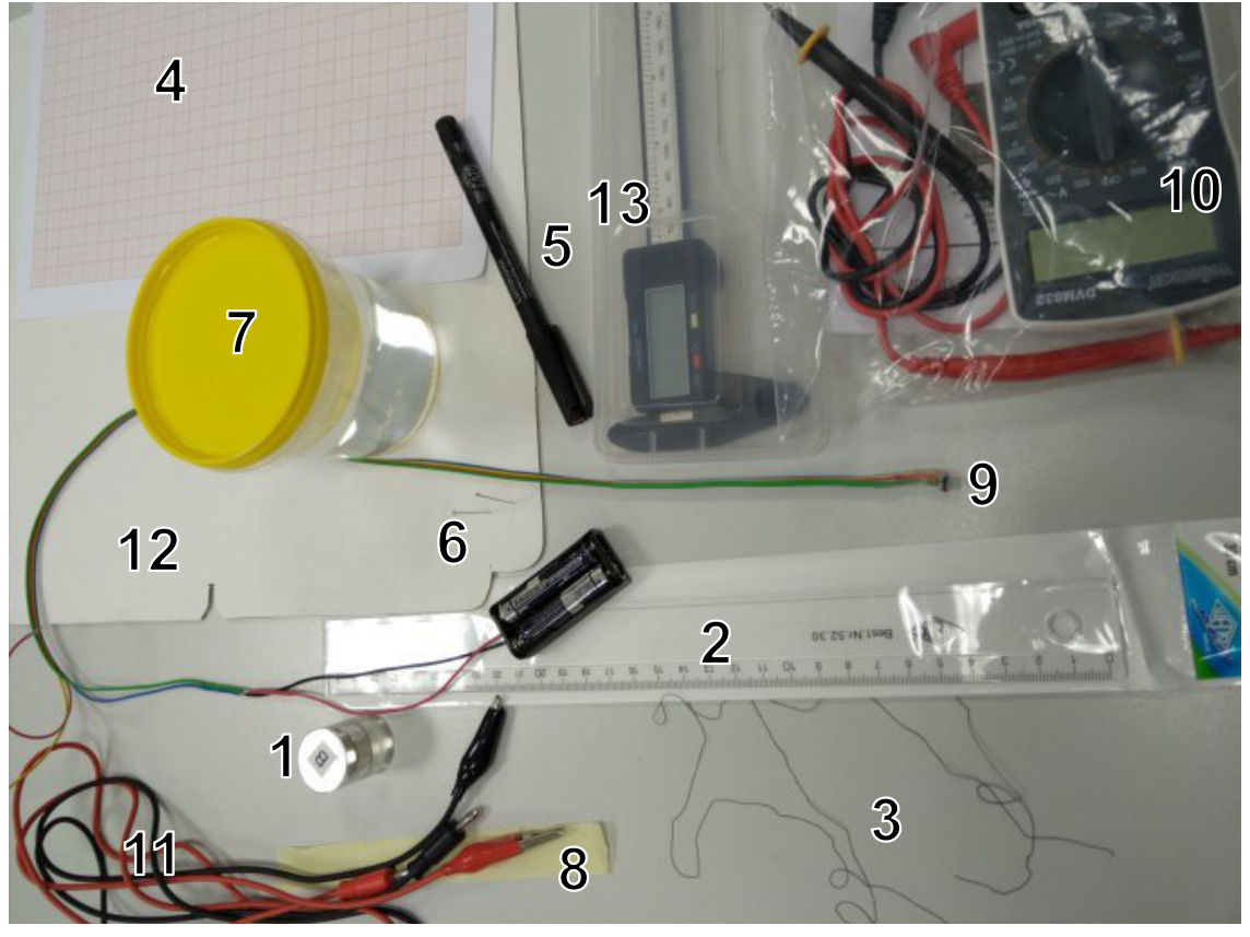
The following equipment is listed in the figure beneath:

1 — a transparent cylinder with a cylindrical permanent magnet inside and with foil caps covering its top and bottom;
2 — a ruler;
3 — a rubber thread;
4 — graph papers;
5 — a permanent marker;
6 — safety pins;
7 — a cup with water;
8 — a tape, for fixing a rubber thread to the cylinder;
9 — a resistive magnetic field sensor connected to batteries in a battery holder;
10 — a multimeter with wires;
11 — two wires with banana/crocodile connectors;
12 — a piece of cardboard, for fixing the safety pins vertically;
13 — a caliper.

WARNINGS:

Avoid short-circuiting the battery leads — the battery will overheat and become unusable!
Power off the multimeter when not in use, in order to conserve the batteries.
Do not peel off the foil caps of the transparent cylinder, even if only partially — if you do, your score will be reduced!
Do not move the magnetic sensor too close to the permanent magnet! If you do, the offset voltage $V_0$ of the sensor may change ( $V_0$ is defined in the problem text.)
Pay attention to the fact that your tables have iron bars beneath. In order to avoid ferromagnetic interference, keep your cylinder and sensor in the middle of the table when doing magnetic measurements.

Tasks

For all the tasks below, keep in mind that parts of the points are given for the precision of your answer, so design and execute your experiments accordingly. Among other things, this might mean doing additional measurements to improve uncertainty estimates (when the task asks for this).

Always draw a sketch showing your measurement setup with clear indications of the positions of all those measurement tools which you are using for the given task. Describe clearly all steps in your solution, a significant amount of points will be given for the adequate procedure, based on your sketches and descriptions. In all cases, write down all the direct measurements results, the formulas used, and the calculations.

A.1 Part A. Geometrical characteristics (5 points)

Find the total volume $V$ of the cylinder and estimate the uncertainty of the result. [2 т.]

A.2 Find the height $h$ of the permanent magnet inside the cylinder and estimate the uncertainty of the result. [1 т.]

A.3 Design such a method for determining the diameter $d$ of the permanent magnet for which knowing the value of the refraction coefficient of the cylinder is not required. Determine the diameter of the magnet and estimate the uncertainty of the result. [2 т.]

Photo of the equipment laid out on a table, with numbered labels 1–13: 1 the transparent cylinder with the magnet, 2 a ruler, 3 a rubber thread, 4 graph paper, 5 a marker, 6 safety pins, 7 a yellow-lidded cup with water, 8 tape, 9 the magnetic field sensor with a battery holder, 10 a multimeter with wires, 11 wires with banana/crocodile connectors, 12 a piece of cardboard, 13 a caliper.

B.1 Part B. Mechanical characteristics (3 points)

Determine the average density of the cylinder (glass with magnet) knowing that the density of water is $\rho_w = 1000\,\mathrm{kg/m^3}$ . [2 т.]

B.2 Determine the total mass of the cylinder. [0,5 т.]

B.3 Determine the average density of the glass knowing that the density of the magnet is $\rho_m = 7500\,\mathrm{kg/m^3}$ . [0,5 т.]

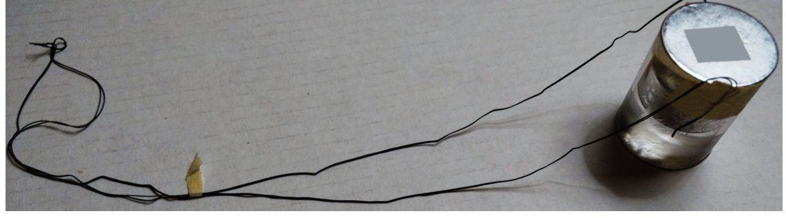
Hint: use the rubber threads as a dynamometer . Join two rubber threads together (to make them stiffer), and, using pieces of tape, attach the ends of the threads to both ends of the cylinder. Also attach a tiny piece of tape to the threads, serving as a marker for taking thread length measurements; the whole setup is shown in the figure below. The tension force in the threads given to you is proportional to the quantity

\tau \equiv \left(1 - \lambda^{-1}\right)\left(1 - 0.2664\lambda + 0.1191\lambda^2\right), \quad \lambda \equiv l/l_0,

where $l$ denotes the length of the thread, and $l_0$ its length in the unstrained state.

Photo of the dynamometer setup: two joined black rubber threads lying on a table, fastened with tape to the transparent cylinder on the right, with a small piece of tape on the threads serving as a length marker.

C.1 Part C. Optical properties (5 points)

Notice that the transparent part of the cylinder is actually made of two different materials: the coefficient of refraction of the central part $n_c$ is slightly different from the coefficient of refraction of the outer part of the cylinder $n_o$ (the central part has the same diameter as the permanent magnet). Design a method for determining the coefficient of refraction $n_o$ and estimate the uncertainty of the result.

Hint: Measure the apparent diameter of the magnet and relate it to the refractive index $n_o$ using Snell’s law. [2,5 т.]

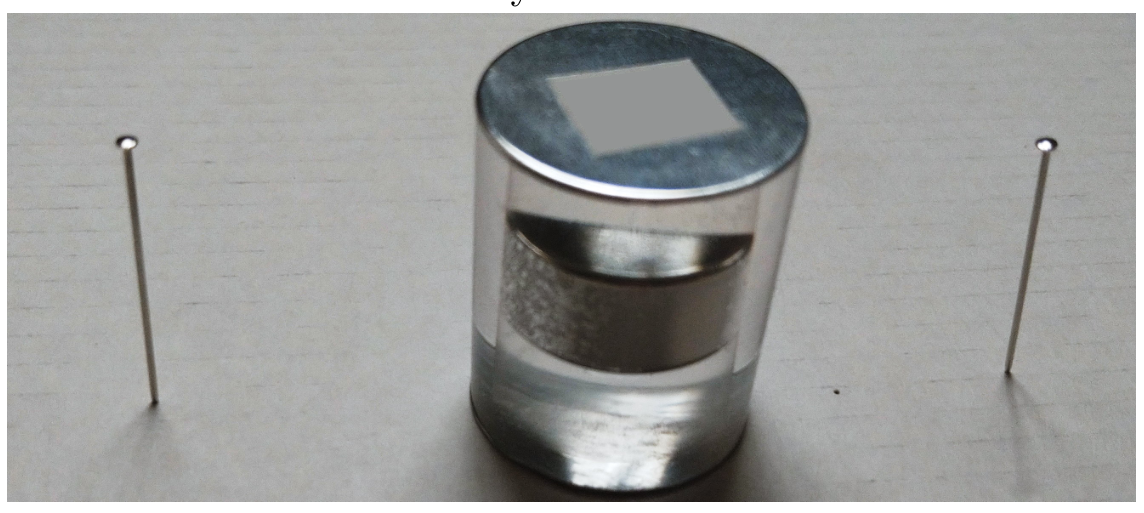
C.2 In order to determine the coefficient of refraction $n_c$ , you are asked to use the cylinder as a thick lens, and create with it an image of a safety pin, and to use the parallax method for determining the position of the pin’s image. To that end, complete the following steps, the end result of which is shown below. Fix two safety pins vertically into the provided piece of cardboard, such that the distance between the pins is bigger than the diameter of the cylinder. Place the cylinder vertically between the two pins such that the distances from both of the pins to the cylinder are strictly equal and such that the pins and the axis of the cylinder lie on the same line $s$ . Look at the cylinder from the side of one of the pins, along the line $s$ — so that the pin closer to you (let us call this pin “the pin A”) will overlap the image of the other pin — the pin B, as seen through the cylinder. Now, move your head (eye) rightwards; if the pin A moves rightwards from the image of the pin B, it means that it is farther away from you than the image of the pin B. You need to achieve the situation where pin A and the image of pin B coincide: in that case, their relative position will not change when you move your eye leftwards or rightwards from the initial position. You will need to pull the pins out and move them farther away from each other, or move them closer as needed, while maintaining an equal distance between the pins and the cylinder, and repeat it until the desired result has been achieved. Measure the distance $L$ between the two pins on the cardboard once pin A and the image of pin B coincide and estimate the uncertainty of the result. [1,5 т.]

Photo of the transparent cylinder with the dark magnet visible inside, standing upright between two vertical safety pins stuck into cardboard, one pin on each side at equal distances.

C.3 Determine the coefficient of refraction $n_c$ of the cylinder.

Hint: you may use the formula

\left(\frac{1}{L-D} - \frac{n_o - 1}{D}\right)\left(\frac{n_c d}{n_c - n_o} - D\right) = n_o,

where $D$ denotes the diameter of the cylinder. [1 т.]

D.1 Part D. Magnetic properties (7 points)

Connect the banana ends of the two wires to the COM port and to the V $\Omega$ mA-port of the multimeter. Switch on the multimeter in 20 volt (DC) range, and touch the two metallic leads of the battery holder (which are next to the points were the red and black wires come out from the holder) with the crocodile ends of the wires. Record the voltage $\mathcal{E}$ on the output leads of the battery holder. If the voltage is below $3.0\,\mathrm{V}$ , you may ask for replacement batteries. [0,5 т.]

For all your magnetic field measurements, keep in mind that if the battery voltage were to be exactly $3\,\mathrm{V}$ , each millivolt in the reading would correspond to 10 microteslas of the magnetic field strength. However, the reading in millivolts is proportional to both the magnetic field and to the battery voltage. So, to calculate the magnetic field strengths, you will be needing this battery voltage value.

Connect the crocodiles to the yellow and red wires of the magnetic sensor. Keep in mind that the sensor may have a non-zero offset: even if there is no magnetic field, the multimeter reading $V_0$ might be non-zero. You should also keep in mind that there is always the magnetic field of Earth.

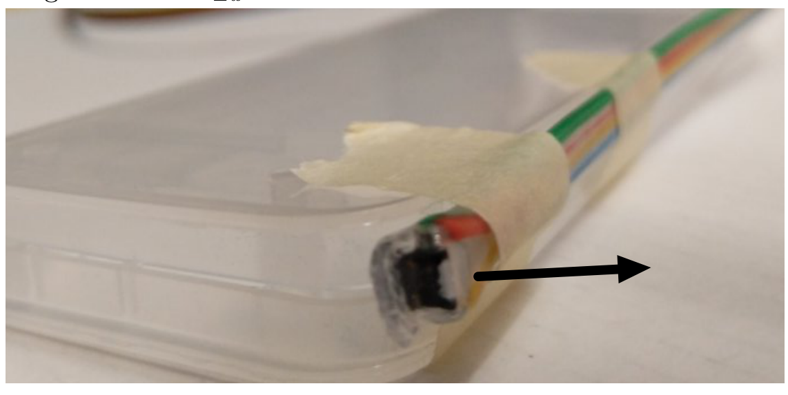
D.2 Let the $x$ -axis be horizontal and parallel to the shorter edge of your desk. From this part onwards, we measure only the $x$ -component of the magnetic fields. It is convenient to fix the magnetic sensor to the plastic box of the caliper with pieces of tape as shown in the figure below: with such a setup the orientation of the sensor can be easily kept unchanged. The arrow in the figure shows the direction of the measured magnetic field component.

Switch on the multimeter in 200 millivolt (DC) range, put the sensor on the table far away from the magnet so that it will measure the $x$ -component of the magnetic field, take the reading of the multimeter $V_1$ , and write it down. Turn the sensor by 180 degrees (so that it will again measure the $x$ -component of the magnetic field, but in the opposite direction), and take the new reading $V_2$ . Based on these two readings, determine the offset voltage $V_0$ , and the horizontal component of the Earth’s magnetic field $B_{Ex}$ . [1 т.]

Close-up photo of the small magnetic sensor fixed with tape to the edge of the caliper's plastic box, its multicoloured ribbon cable running away; a black arrow pointing to the right shows the direction of the measured field component.

D.3 Measure and tabulate the $x$ -component of the magnetic field $B_x(x)$ of the permanent magnet for a series of points at different distances $x$ from the centre of the magnet, on the symmetry axis of the magnet (the $x$ -axis). You are expected to take readings for the full usable range of the distances. Avoid distances by which the voltage reading exceeds $300\,\mathrm{mV}$ . Do not forget to report the direct measurement results (the voltages), and when calculating the magnetic field values, to subtract the offset voltage (you need to compensate both for the $x$ -component of the Earth’s magnetic field, and for the non-zero offset voltage $V_0$ ). [2,5 т.]

D.4 If the distance from the magnet is big enough, its strength is given by the formula

B_x(x) = \frac{\mu_0}{2\pi}\frac{p}{x^3},

where $p$ denotes the magnetic dipole moment of the magnet and $\mu_0 = 4\pi \times 10^{-7}\,\mathrm{H\,m^{-1}}$ is the vacuum permeability. Find a way to plot the measurement data from the previous task so that the data points following this formula would lay in a straight line. Show for which values of $x$ , the formula holds within the measurement uncertainties. Use your graph to determine the dipole moment of the magnet. [2,5 т.]

D.5 Find the magnetization $J$ of the permanent magnet (defined as the volume density of the magnetic dipole moment). [0,5 т.]

Отговори

A.1 15.2 ml

Official value $V = (15.2 \pm 0.2)\,\mathrm{ml}$ ; full marks within $[14.8\,\mathrm{ml}, 15.6\,\mathrm{ml}]$ .
A.2 9.5 mm

Official value $h = (9.5 \pm 0.2)\,\mathrm{mm}$ ; full marks within $[9.1\,\mathrm{mm}, 10.0\,\mathrm{mm}]$ .
A.3 12 mm

Official value $d = (12.0 \pm 0.7)\,\mathrm{mm}$ ; full marks within $[11.0\,\mathrm{mm}, 13.0\,\mathrm{mm}]$ .
B.1 1720 kg/m³

Official value $\rho_{\mathrm{cyl}} = 1720\,\mathrm{kg/m^3}$ ; full marks within $[1620, 1820]\,\mathrm{kg/m^3}$ .
B.2 26.1 g

Official value $m_{\mathrm{cyl}} = 26.1\,\mathrm{g}$ ; full marks within $[25.0\,\mathrm{g}, 27.1\,\mathrm{g}]$ .
B.3 1280 kg/m³

Official value $\rho_g = 1280\,\mathrm{kg/m^3}$ ; full marks within $[1130, 1430]\,\mathrm{kg/m^3}$ .
C.1 1.54

Official value $n_o = 1.54$ , $\Delta n_o = 0.09$ ; full marks within $[1.50, 1.58]$ .
C.2 62.1 mm

Official value $L = 62.1\,\mathrm{mm}$ , $\Delta L = 0.5\,\mathrm{mm}$ ; full marks within $[61.1\,\mathrm{mm}, 63.1\,\mathrm{mm}]$ .
C.3 1.6

Official value $n_c = 1.60$ ; full marks within $[1.55, 1.65]$ .
D.1 3.15 V

Official measurement $\mathcal{E} = 3.15\,\mathrm{V}$ (depends on the batteries provided).
D.2 V0 = −0.8 mV, BEz = 23 µT

Official readings $V_1 = 1.4\,\mathrm{mV}$ , $V_2 = -2.9\,\mathrm{mV}$ ; the official solution denotes the Earth's field component $B_{Ez}$ .
D.4 1.4 A m²

Official value $p = 1.40\,\mathrm{A\,m^2}$ from the slope $A = 0.0153\,\mu\mathrm{T^{-1/3}\,cm^{-1}}$ of $B_x(x)^{-1/3}$ vs $x$ .
D.5 $1.3 \times 10^{6}$ A/m

Official value $J = 1.30 \times 10^6\,\mathrm{A\,m^{-1}}$ ; full marks within $1.1 \times 10^6 \le J \le 1.4 \times 10^6\,\mathrm{A\,m^{-1}}$ .

Решение

Problem E1. Cylinder in cylinder (20 points)

Part A. Geometrical characteristics (5 points)

1. (2 pts) We can find the total volume by using the caliper to measure the base diameter $2R$ and the total height $H$ of the cylinder via

V = \pi R^2 H.

Two concentric circles (outer radius R, inner radius r of the magnet). A ray enters the outer circle from below, runs as a straight chord tangent to the inner circle and exits at the upper right; the chord half-length is labelled a/2, the dashed radius to the exit point is labelled R, and the dashed radius to the tangent point is labelled r with a right-angle mark. — Figure 1: Optics of the cylinder

(0.4 pts)

The values were measured to be

$i$	$2R$ (mm)	$H$ (mm)
1	25.2	30.4
2	25.0	30.5
3	25.3	30.5
3	25.1	30.4
3	25.3	30.5

1 diameter measurement (0.3/0.5 pts)
2 diameter measurements (0.4/0.5 pts)
3 or more diameter measurements (0.5/0.5 pts)

1 or more height measurement (0.3/0.3 pts)

Each measurement carries its own uncertainty of that of a caliper $\Delta l = 0.2\,\mathrm{mm}$ . Based on this, we calculate $R = (12.6 \pm 0.1)\,\mathrm{mm}$ , $H = (30.5 \pm 0.2)\,\mathrm{mm}$ and $V = (15.2 \pm 0.2)\,\mathrm{ml}$

value within $[14.8\,\mathrm{ml}, 15.6\,\mathrm{ml}]$ (0.4 pts)
error (0.4 pts)

2. (1 pt) The height is best measured using a caliper by either making markings on the surface of the cylinder corresponding to the perpendiculars of the ends of the magnet, or by measuring it from far away. Either way, the goal is to remove the effects of parallax when measuring the height of the cylinder. The following measurements were made

$i$	$h$ (mm)
1	9.7
2	9.5
3	9.4

1 measurement (0.3/0.5 pts)
2 measurements (0.4/0.5 pts)
3 or more measurements (0.5/0.5 pts)

The average height is found to be $h = (9.5 \pm 0.2)\,\mathrm{mm}$ .

value within $[9.1\,\mathrm{mm}, 10.0\,\mathrm{mm}]$ (0.3 pts)
error (0.2 pts)

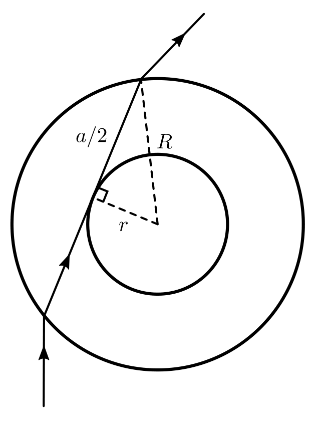
3. (2 pts) A potential method would be to observe the light ray that barely touches the edge of the magnet, (0.4 pts) and make markings where the ray enters and exits the cylinder. This works, because the markings define a chord whose distance from the centre is the radius of the magnet $r = d/2$ . Hence, the distance between the markings $a$ relates to $r$ and $R$ via Pythagoras theorem via $r = \sqrt{R^2 - a^2/4}$ or in other words,

d = \sqrt{4R^2 - a^2}.

(0.6 pts)

Figure 1: Optics of the cylinder

We make the following measurements for $a$ :

$i$	$a$ (mm)
1	22.2
2	22.5
3	21.8

1 measurement (0.3/0.5 pts)
2 measurements (0.4/0.5 pts)
3 or more measurements (0.5/0.5 pts)

This yields $a = (22.2 \pm 0.3)\,\mathrm{mm}$ such that $d = (12.0 \pm 0.7)\,\mathrm{mm}$ .

value within $[11.0\,\mathrm{mm}, 13.0\,\mathrm{mm}]$ (0.3 pts)
error (0.2 pts)

Part B. Mechanical characteristics (3 points)

1. (2 pts) We can make a makeshift scale by attaching the cylinder to a rubber thread and measuring how much it extends. The force exerted by the thread is then equal to the Archimedes force of the cylinder and proportional to $\tau(l/l_0$ given in the problem statement.

Knowing the water density, it would satisfy us to measure the length of the attached thread when the cylinder is submerged $l_w$ , when it’s not $l_a$ and finally when it’s at rest (cylinder isn’t attached), $l_0$ . (0.3 pts)

Using Archimedes’ law, the quantities then satisfy

\begin{aligned} k\tau(l_a/l_0) &= V\rho_{\mathrm{cyl}}g,\\ k\tau(l_w/l_0) &= V(\rho_{\mathrm{cyl}} - \rho_w)g, \end{aligned}

(0.4 pts)

where $k$ is a constant and the left hand side corresponds to the tension force of the rubber threads. Thus,

\rho_{\mathrm{cyl}} = \rho_w \frac{\tau(l_a/l_0)}{\tau(l_a/l_0) - \tau(l_w/l_0)}.

(0.2 pts)

We proceed to make one set of measurements (as estimating uncertainties isn’t necessary) and get $l_0 = 135\,\mathrm{mm}$ , $l_a = 303\,\mathrm{mm}$ , $l_w = 185\,\mathrm{mm}$ . (0.6 pts)
Thus, we calculate $\tau(l_a/l_0) = 0.556$ , $\tau(l_w/l_0) = 0.232$ and so $\rho_{\mathrm{cyl}} = 1720\,\mathrm{kg/m^3}$ .

Two concentric circles (outer and inner). A vertical ray comes up from below at horizontal distance r′ from the centre, refracts at the outer circle and continues tangent to the inner circle, then exits at the upper right. The angle of incidence α with the dashed normal and the refraction angle β are marked; dashed segments show the radius R to the entry point, the radius r to the tangent point with a right-angle mark, and the horizontal distance r′ at the bottom. — Figure 2: Detailed optics of the cylinder

value within $\left[1620\,\mathrm{kg/m^3}, 1820\,\mathrm{kg/m^3}\right]$ (0.3 pts)

2. (0.5 pts) The total mass of the cylinder is simply found as $m_{\mathrm{cyl}} = V\rho_{\mathrm{cyl}} = 26.1\,\mathrm{g}$ .

formula (0.3 pts)
value within $[25.0\,\mathrm{g}, 27.1\,\mathrm{g}]$ (0.2 pts)

3. (0.5 pts) We can express the total mass of the cylinder as a sum of the mass of the magnet and the glass surrounding the magnet:

m_{\mathrm{cyl}} = h\pi r^2\rho_m + (H\pi R^2 - h\pi r^2)\rho_g.

(0.2 pts)

Thus, glass’ density is

\rho_g = \frac{\rho_{\mathrm{cyl}}HR^2 - \rho_m h r^2}{HR^2 - hr^2} = 1280\,\mathrm{kg/m^3}.

formula (0.1 pts)
value within $\left[1130\,\mathrm{kg/m^3}, 1430\,\mathrm{kg/m^3}\right]$ (0.2 pts)

Part C. Optical properties (5 points)

1. (2.5 pts) The most direct method would be to measure how much the magnet appears to be bigger than its actual width.

Showing or stating the method or idea in text or graphically (0.5 pts)

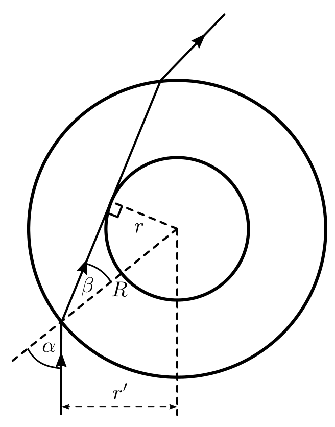
The optics of this is shown on figure 2. On the figure, $r'$ is the apparent radius of the magnet when the cylinder is observed from far away. In practice, one could measure the apparent diameter $d' = 2r'$ using a caliper and a marker.

Figure 2: Detailed optics of the cylinder

Carrying out the method or idea correctly (0.25 pts)

From the figure, we work out from Snell’s law that $\sin\alpha = n_o \sin\beta$ , but from right triangles $\sin\beta = r/R$ and $\sin\alpha = r'/R$ . Hence, $n_o = r'/r = d'/d$ .

Stating and applying Snell’s law correctly (0.5 pts)

Tabulated measurements of the apparent width are shown below

$i$	$d'$ (mm)
1	18.3
2	18.5
3	18.8

3 or more measurements (0.3 pts)
with units (0.2 pts)

Averaging, $d' = (18.5 \pm 0.4)\,\mathrm{mm}$

average value of d with errors (0.25 pts)

and so $n_o = 1.54$ with an associated error of $\Delta n_o = 0.09$ .

value within $[1.50, 1.58]$ (0.25 pts)
error (0.25 pts)

2. (1.5 pts) Constructing the optical system described in the task statement, we make the following measurements

$i$	$L$ (mm)
1	62.7
2	61.1
3	62.0
4	62.6
5	62.2

3 or more measurements (0.3 pts)
with units (0.2 pts)

Averaging, we find $L = 62.1\,\mathrm{mm}$ with an error of $\Delta L = 0.5\,\mathrm{mm}$ .

Value with units within $[61.1\,\mathrm{mm}, 63.1\,\mathrm{mm}]$ (0.5 pts)
Error (0.5 pts)

3. (1 pt) Starting from the formula

\left(\frac{1}{L-D} - \frac{n_o - 1}{D}\right)\left(\frac{n_c d}{n_c - n_o} - D\right) = n_o,

we find

n_c = n_0\left(1 - \frac{d}{D + \frac{n_0}{\frac{1}{L-D} - \frac{n_0 - 1}{D}}}\right)^{-1} = 1.60.

Starting from previous equation of $n_0$ and showing the steps of algebraic manipulation to arrive at $n_c$ (0.7 pts)
value within $[1.55, 1.65]$ (0.3 pts)

Part D. Magnetic properties (7 points)

1. (0.5 pts) We measure $\mathcal{E} = 3.15\,\mathrm{V}$ . Any value above $3.20\,\mathrm{V}$ or $3.00\,\mathrm{V}$ will give 0 points. Missing units: subtract 0.2 points.

2. (1 pt) We measure $V_1 = 1.4\,\mathrm{mV}$ and $V_2 = -2.9\,\mathrm{mV}$ . (0.2 pts)

(No points are awarded if only $V_1$ or $V_2$ are measured or voltages readings are incorrect. Reading is judged to be incorrect if the corresponding magnetic field (when calculated correctly) would be greater than $50\,\mu\mathrm{T}$ .)

The voltage is affected by the offset voltage and the Earth’s magnetic field $B_{Ez}$ . The Earth’s magnetic field influences the reading by a voltage offset $V_{Ez} = B_{Ez}/a$ , where $a$ is a constant. We know that if the battery voltage were to be $3\,\mathrm{V}$ , then each millivolt is $10\,\mu\mathrm{T}$ . Our battery increases the scaling by a factor of $\mathcal{E}/3\,\mathrm{V}$ . In other words, to convert from volts to microteslas, we multiply our voltage through by $a = 10\,\mu\mathrm{T/V} \cdot \mathcal{E}/3\,\mathrm{V} = 10.5\,\mu\mathrm{T/V}$ .

Taking all this together, we have $V_1 = V_0 + B_{Ez}/a$ and $V_2 = V_0 - aB_{Ez}$ and so $V_0 = (V_1 + V_2)/2$ , (0.2 pts)

B_{Ez} = (V_1 - V_2)a/2.

(0.1 pts)

Numerically we get $V_0 = -0.8\,\mathrm{mV}$ , (0.1 pts)

B_{Ez} = (V_1 - V_2)a/2 = 23\,\mu\mathrm{T}.

(0.4 pts)

For this magnetic field value, no points are given if its calculation has mistakes (i.e. it does not correspond to the reported voltage values). If $a = 10.0\,\mu\mathrm{T/V}$ was used even though the voltage was not $3.00\,\mathrm{V}$ , 0.2 point will be subtracted.

3. (2.5 pts) We measure the sensor voltage throughout the full measurement range, from the end of the ruler at $30\,\mathrm{cm}$ up to when voltage reaches $300\,\mathrm{mV}$ . To convert to magnetic field, we first offset the measured voltage $V$ to remove the bias and the contribution from the magnetic field. This corresponds to subtracting $V_1$ due to the orientation of the sensor. Finally, we divide by $a$ to get the magnetic field, i.e. $B_x(x) = (V - V_1)/a$ . The tabulated data is given below.

$l$ (cm)	$x$ (cm)	$V$ (mV)	$B_x(x)$ ( $\mu$ T)	$B_x(x)^{-1/3}$ ( $\mu\mathrm{T}^{-1/3}$ )
30	30.5	2.5	11.6	0.442
25	25.5	3.0	16.8	0.390
22	22.5	3.5	22.1	0.357
20	20.5	4.2	29.4	0.324
19	19.5	4.7	34.7	0.307
18	18.5	5.4	42.0	0.288
17	17.5	6.2	50.4	0.271
16	16.5	7.0	58.8	0.257
15	15.5	8.3	72.5	0.240
14	14.5	9.9	89.3	0.224
13	13.5	12.3	115	0.206
12	12.5	15.4	147	0.189
11	11.5	19.9	194	0.173
10	10.5	26.2	260	0.156
9	9.5	35.4	357	0.141
8	8.5	48.5	495	0.126
7	7.5	70.0	720	0.112
6	6.5	108	1120	0.096
5	5.5	178	1850	0.081

$l$ is the distance from the face of the magnet and hence, to get the distance from the centre of the magnet $x$ , we need to offset it by half of the thickness of the magnet $h/2 = 0.5\,\mathrm{cm}$ . The table features an additional column that’s used in the next subtask.

For each voltage value until 10th data point: (0.1 pts)
Datapoints at $l < 4\,\mathrm{cm}$ are not counted
For each calculated $B_x$ value until 10th data point: (0.1 pts)
Calculations at $l < 4\,\mathrm{cm}$ are not counted
For a reading taken at $4\,\mathrm{cm} \le l < 6\,\mathrm{cm}$ (0.1 pts)
For a reading taken at $6\,\mathrm{cm} \le l < 8\,\mathrm{cm}$ (0.1 pts)
For a reading taken at $l > 25\,\mathrm{cm}$ (0.1 pts)
For a reading taken at $25\,\mathrm{cm} \ge l > 20\,\mathrm{cm}$ (0.1 pts)
For a reading taken at $20\,\mathrm{cm} \ge l > 15\,\mathrm{cm}$ (0.1 pts)

Marks are not given for obviously wrong voltage values and for $B_x$ values which differ from correct values by more than 20% plus $10\,\mu\mathrm{T}$ .

If offset is not subtracted, multiply the score for taken readings by 0.5.

4. (2.5 pts)

If the magnetic field is given by

B_x(x) = \frac{\mu_0}{2\pi}\frac{p}{x^3},

we can linearize it in many different ways, but a convenient way would be to consider $B_x(x)^{-1/3}$ vs $x$ as that maintains the linear spacing of the data points. In that case,

B_x(x)^{-\frac{1}{3}} = \sqrt[3]{\frac{2\pi}{\mu_0 p}}\,x = Ax,

where the slope gives us $p$ via $p = 2\pi/(\mu_0 A^3)$ . We calculate $B_x(x)^{-1/3}$ and plot it, shown below.

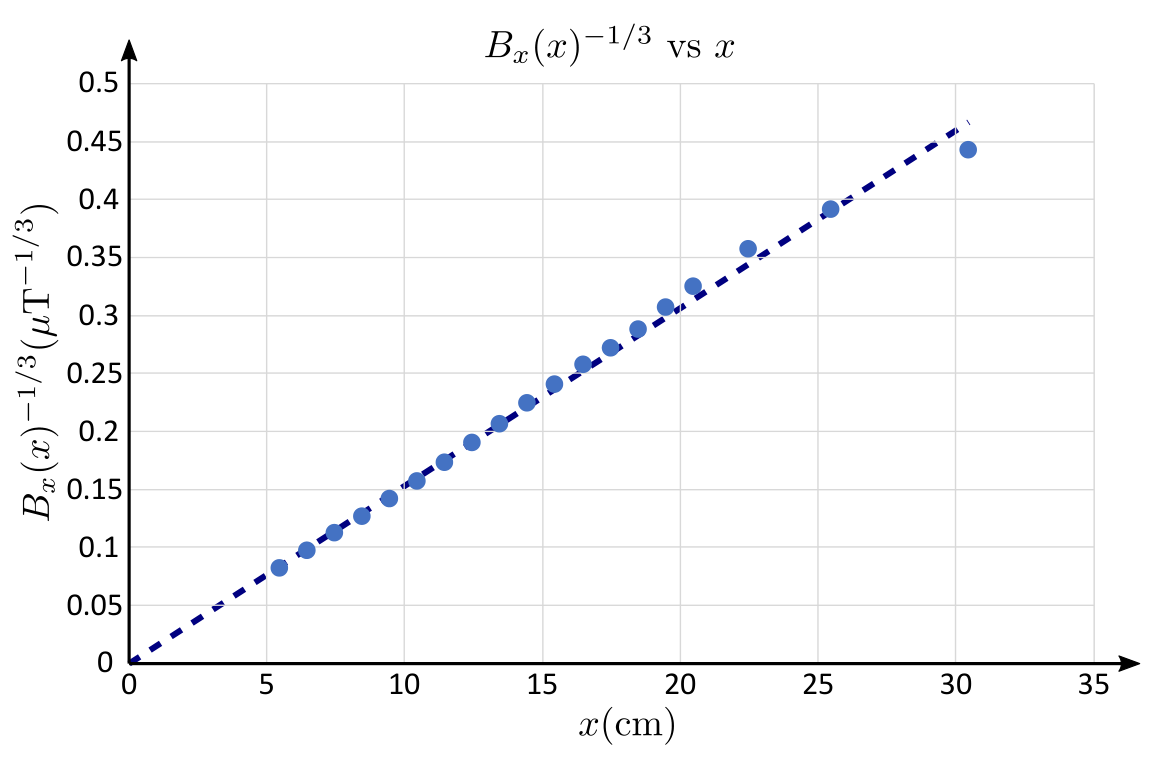
Graph titled “$B_x(x)^{-1/3}$ vs $x$”: vertical axis $B_x(x)^{-1/3}$ ($\mu\mathrm{T}^{-1/3}$) from 0 to 0.5, horizontal axis x(cm) from 0 to 35; blue data points from x ≈ 5.5 to 30.5 cm lie close to a dashed straight line through the origin, the last point at x ≈ 30.5 falling slightly below the line.

From the graph, we measure $A = 0.0153\,\mu\mathrm{T}^{-1/3}\,\mathrm{cm}^{-1} = 153\,\mathrm{T^{-1}\,m^{-1}}$ so

p = \frac{2\pi}{\mu_0 A^3} = 1.40\,\mathrm{A\,m^2}.

Suitably chosen quantities on axis (which makes the graph linear) (0.5 pts)
For each data point up to the tenth, calculation of the value for the vertical axis with correct plotting (0.1 pts)
If points are not marked on a plot, only half marks are given.
If $B_x$ values are directly plotted, only half marks are given.
Finding the slope of the linear part of the graph (0.3 pts)
Numerical calculation of $p$ (0.2 pts)

5. (0.5 pts) From the definition, magnetization is

J = \frac{p}{\pi r^2 h} = 1.30 \times 10^6\,\mathrm{A\,m^{-1}}.

Correct value $1.1 \times 10^6\,\mathrm{A\,m^{-1}}J \le J \le 1.4 \times 10^6\,\mathrm{A\,m^{-1}}$ (0.5 pts)

Оригинал в Архива: exp.pdf · официални решения: exp_sol.pdf