Съдържание

IAO 2007, Практически тур, Група α — Задача 6. The O-C diagram.

Оригинал на условието (изображение)Съобщи за грешка

Всички материали от IAO 2007

Practical round. Problems to solve · 29 септември 2007 г.

Note for jury and team leaders

Note for jury and team leaders. The proposed sketches are not full; the team leaders have to give more detailed explanations for students. But the correct solutions in the students’ papers (enough for 10pts) may be shorter.

Source annotations

The official O−C answer table prints calculated dates47685 and47383 for observations12 and13 respectively; these do not agree with the surrounding cycle sequence or the printed O−C values. The first interval in its final table is printed0–45878.2. All these printed entries are retained without correction.

Условие

Variable stars of the Mira Cetus type show significant variations in their pulsational period from cycle to cycle. Sometimes their periods increases or decreases during a long time period, sometimes it suddenly changes from one value to another, or show irregular variation. In addition to this, the shape of the light curve can change, and this leads to irregular errors in the determination of the moments of maximum of the light. To find a possible period variation, so called «O-C» diagrams are used. They give the dependence of the difference between observed (O) and calculated (C) moments of maximum light upon JD or cycle number. The moment of maximum is calculated using the linear formula $T=T_0+PE$ , where $T_0$ is some initial moment of maximum, $P$ is the supposed period, $E$ is the number of cycles that passed after the moment $T_0$ . The two columns of the table list the observational data, the number of current of observation, and corresponding moment of maximum O for a certain star of the considered type.

For this star the value of the calculated period determined before the listed observations was 302.0 days.

N of observation	JD 244.... (O)
1	42551.0
2	42852.1
3	43155.8
4	44063.3
5	44365.5
6	44969.9
7	45273.9
8	45878.2
9	46181.8
10	46486.4
11	46791.2
12	47401.9
13	47706.2
14	48007.4
15	48308.1
16	48609.5
17	48909.4
18	49210.8
19	49811.8
20	50114.6
21	50414.5

6.1.

Fill in the empty spaces of the table (at the separate sheet).

N	JD 244.... (O)	E	O−C
1	42551.0	0	0
2	42852.1
3	43155.8
4	44063.3
5	44365.5
6	44969.9
7	45273.9
8	45878.2
9	46181.8
10	46486.4
11	46791.2
12	47401.9
13	47706.2
14	48007.4
15	48308.1
16	48609.5
17	48909.4
18	49210.8
19	49811.8
20	50114.6
21	50414.5

6.2.

Make a plot “O-C” versus E.

6.3.

Using the “O-C” diagram find the regions where the period is relatively stable (i.e. it changes not very significantly from cycle to cycle), and find the mean value $\langle P\rangle$ for each of these time intervals. In your copybook make a new table (see an example at right side) in which each line should contain the corresponding intervals of the relatively stable periods and its approximate value.

Region, NN	Interval JD 244.... – JD 244....	$\langle P\rangle$

Решение

Use the given value of period $P=302.0^{\mathrm d}$ we can calculate «O-C» values for all the moments of maximum light and fill in the big table. It should be taken into account that not all maximums were observed. So the number of cycle E is not equal to the number of the moment of maximum given in the table.

N	JD 244.... (O)	JD 244.... (C)	E	O−C
1	42551.0	42551	0	0
2	42852.1	42853	1	-0,9
3	43155.8	43155	2	0,8
4	44063.3	44061	5	2,3
5	44365.5	44363	6	2,5
6	44969.9	44967	8	2,9
7	45273.9	45269	9	4,9
8	45878.2	45873	11	5,2
9	46181.8	46175	12	6,8
10	46486.4	46477	13	9,4
11	46791.2	46779	14	12,2
12	47401.9	47685	16	18,9
13	47706.2	47383	17	21,2
14	48007.4	47987	18	20,4
15	48308.1	48289	19	19,1
16	48609.5	48591	20	18,5
17	48909.4	48893	21	16,4
18	49210.8	49195	22	15,8
19	49811.8	49799	24	12,8
20	50114.6	50101	25	13,6
21	50414.5	50403	26	11,5

Using the data from this table we can plot «O-C» versus the number of cycle E:

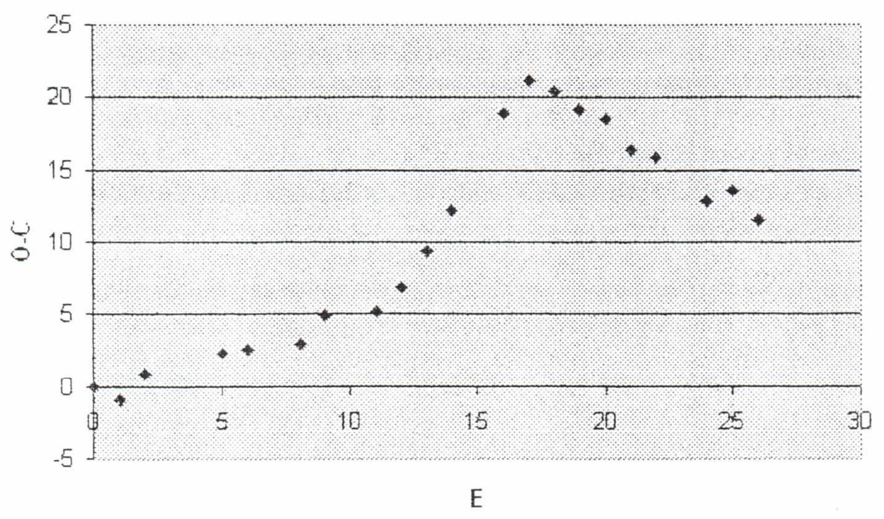
There are three regions on the plot where the experimental points may be approximated by lines, the real period of pulsation in these regions slightly changes from cycle to cycle but is stable in general. These three regions are separated by sudden period change points near E=11 and E=17.
The mean pulsational period for each of the three zones can be found as calculated period plus tan(inclination angle) of the approximational curve. The filled table is below:

E	ΔJD	$\langle P\rangle$
0–11	0–45878.2	302.75
11–17	45878.2–47706.2,	304.3
17–26	47706.2–50414.5	301.04

Оригинал в Архива: alphapract1.jpg · официални решения: practsol1.jpg · допълнителни данни: alphapract2.jpg · допълнителни данни: alphapractdata.jpg · допълнителни данни: practsol2.jpg