Съдържание

INPhO 2025, Теория — Задача 4. The Magnetic Black Box (MBB)

Оригинал на условието (PDF)Съобщи за грешка

Всички материали от INPhO 2025

Indian National Physics Olympiad (INPhO)-2025 — Question Paper · 2 февруари 2025 г. · 22 т.

Внимание: Бележка към темата

The complete retained original question and matching HBCSE solution packets are transcribed. The separately referenced Answer Booklet is not retained in the matching archive row. Printed key formula/sign/symbol/prose discrepancies and the original handwritten magnetic-data graph remain literal, with separately labelled source notes.

Original cover and instructions

Indian National Physics Olympiad (INPhO)-2025

HOMI BHABHA CENTRE FOR SCIENCE EDUCATION

Tata Institute of Fundamental Research

V. N. Purav Marg, Mankhurd, Mumbai, 400 088

Question Paper

Date: 02 February 2025

Time: 09:00-12:00 (3 hours)

Maximum Marks: 75

Instructions — Roll Number: $\square\square\square\square-\square\square\square\square-\square\square\square\square$

This booklet consists of 9 pages and total of 5 questions. Write roll number at the top wherever asked.
Booklet to write the answers is provided separately. Instructions to write the answers are on the Answer Booklet.
Non-programmable scientific calculators are allowed. Mobile phones cannot be used as calculators.
Please submit the Answer Sheet at the end of the examination. You may retain the Question Paper.

Question Number	1	2	3	4	5	Total
Maximum Marks	8	14	16	22	15	75

Table of Constants

Speed of light in vacuum	$c$	$3.00\times10^8\ \mathrm{m\cdot s^{-1}}$
Magnitude of electron charge	$e$	$1.60\times10^{-19}\ \mathrm C$
Value of $1/4\pi\epsilon_0$		$9.00\times10^9\ \mathrm{N\cdot m^2\cdot C^{-2}}$
Avogadro’s number	$N_A$	$6.022\times10^{23}\ \mathrm{mol^{-1}}$
Acceleration due to gravity	$g$	$9.81\ \mathrm{m\cdot s^{-2}}$
Universal Gas Constant	$R$	$8.31\ \mathrm{J\cdot K^{-1}\cdot mol^{-1}}$
	$R$	$0.0821\ \mathrm{l\cdot atm\cdot mol^{-1}\cdot K^{-1}}$
Boltzmann constant	$k_B$	$1.3806\times10^{-23}\ \mathrm{J\cdot K^{-1}}$
Permeability constant	$\mu_0$	$4\pi\times10^{-7}\ \mathrm{H\cdot m^{-1}}$

Native key notice

The matching key repeats the cover, constant table, marks table and four instructions with “24 pages” and the title “Solutions”.

Please note that alternate/equivalent methods and different ways of expressing final solutions may exist. A correct method will be suitably awarded.

Условие

A magnetometer is a Hall-effect-based sensor that measures the magnetic field at its location. In the figure below, a magnetometer is located somewhere inside a closed “magnetic black box” (which we shall henceforth refer to as MBB) of negligible thickness. Fig. (1) gives a top view, where the red rectangle depicts the MBB. The plane of the rectangle is taken as the $x$ – $y$ plane of coordinates, with the origin O taken at the top right corner. The unknown location of the magnetometer is denoted by the coordinates $(x_0,y_0)$ . For example, it could be located at the position marked by $\odot$ inside the MBB. Note that the actual location of the magnetometer inside the MBB may be different from that in the figure; this is true for all subsequent figures in this problem as well.

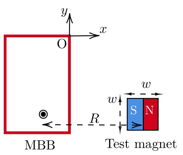
Whole original MBB/test magnet with O/xy/R/w/NS/sensor-location symbols. — Figure 1: Schematic representation of the magnetic black box (MBB) and a test magnet.

The components $B_x,B_y$ and $B_z$ of the magnetic field measured by the magnetometer depend on the strength and the orientation of the magnetic dipole moment, of a magnet positioned nearby and the distance $R$ between the center of the magnet and the magnetometer. The effect of the Earth’s magnetic field is neglected throughout this problem.

Vanya is performing an experiment using the MBB. She has to first locate the exact position of the magnetometer inside the MBB. She has a cubical test magnet of side length $w=10\ \mathrm{mm}$ (see Fig. (1)) and unknown dipole strength $\vec P$ .

She places the MBB on a wooden table. Then she records the magnetic field values displayed by the magnetometer as the test magnet is moved either parallel to the $y$ -axis while keeping $x$ fixed (vertical scan) or parallel to the $x$ -axis while keeping $y$ fixed (horizontal scan) as shown in Fig. (2). The magnitudes of the distances, $r_x$ and $r_y$ , measured from the center of the magnet, are also shown in the figure.

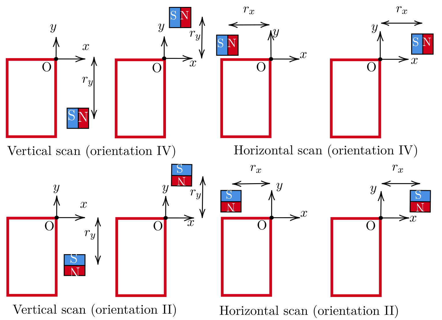
All eight native top-view scan configurations, r_x/r_y/x/y/O and four orientation captions. — Figure 2: Some of the configurations of the vertical and horizontal scans as seen from the top. See Fig. (3) for the explanation of orientations.

For each scan, Vanya also tries different orientations of the magnet by aligning the dipole moment vector $\vec P$ either parallel or anti-parallel to the $y$ -axis or $x$ -axis. The different orientations (I to IV) are shown in Fig. (3). During the experiment, assume that the magnetometer location and the magnet’s center are at the same height (i.e., their $z$ -coordinates are always the same).

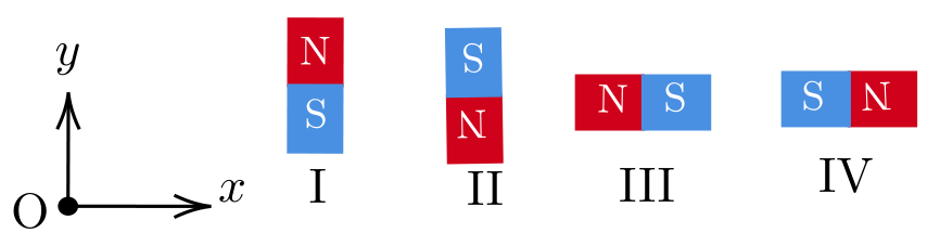
Four native magnet orientations I–IV with N/S blocks and O/xy axes. — Figure 3: Different orientations of the test magnet

The graphs in Fig. (4) display the variation of the magnetic field $B_x$ for four of the vertical and horizontal scans (denoted by A, B, C, D) with certain combinations of the orientations.

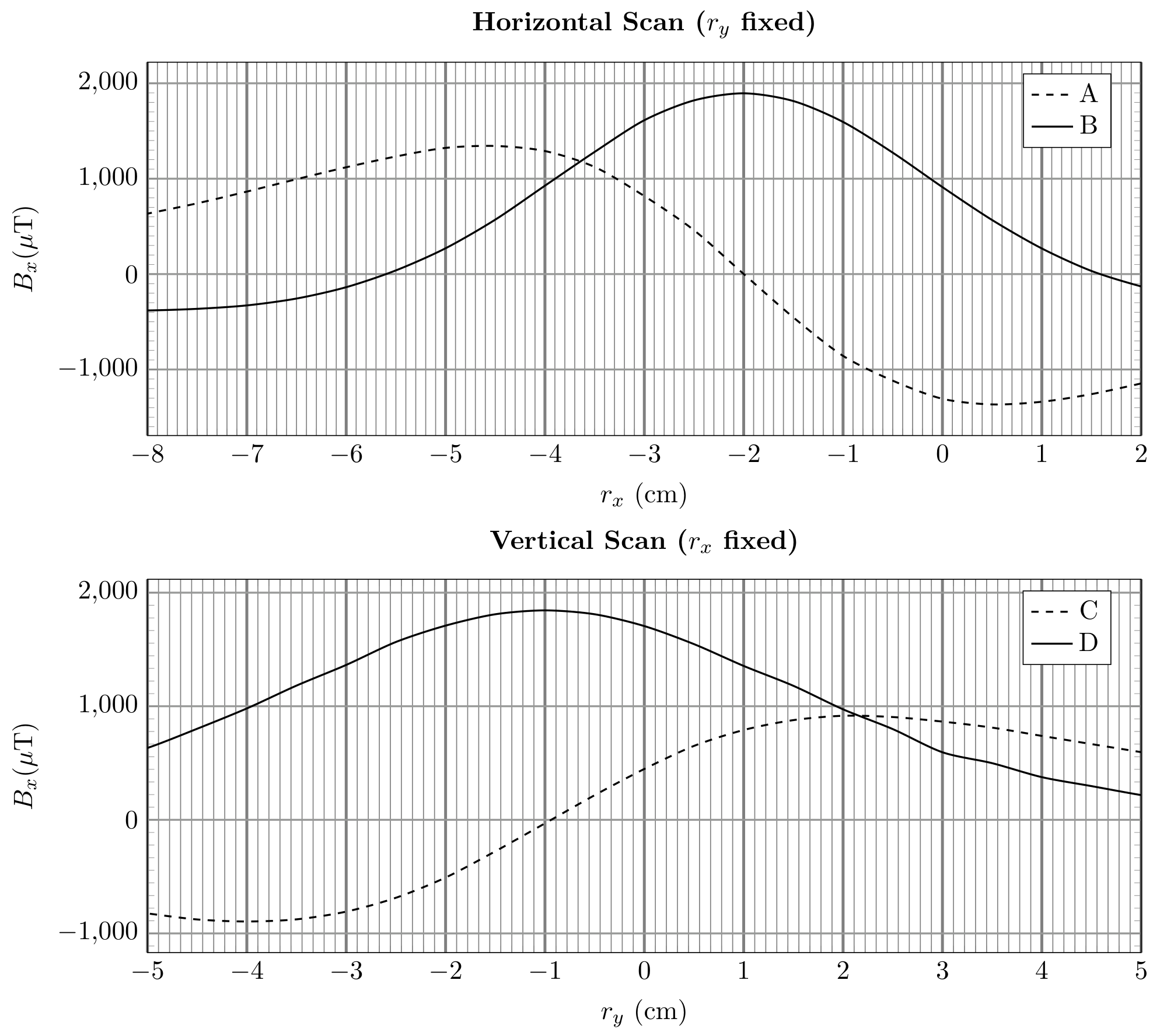
Full horizontal A/B and vertical C/D plots, all gridlines/ticks/units/legends/titles/axes. — Figure 4

a) Based on the above plots, identify which orientations (I-IV) these curves belong to. To indicate your answer, fill in the table in the answersheet. Determine the coordinates $(x_0,y_0)$ of the magnetometer’s position. You must justify your answers. [7 т.]

b) Vanya is given two cuboidal magnetic sets M1 and M2, each constructed using two identical cubic magnets (of side length $w=10\ \mathrm{mm}$ ). In set M1, two magnets, each of dipole moment $P'$ , are joined in an attractive configuration. In set M2, the magnets are joined in a repulsive configuration using a strong adhesive. Thus, each magnetic set has a length of $2w$ (as shown in Fig. (5)).

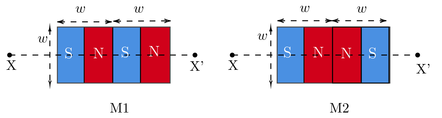
Both native M1/M2 magnetic sets, NS-NS/SN-NS and w/XX-prime labels. — Figure 5: Magnetic sets M1 and M2. Here w = 10mm.

Vanya aligns the central axis (XX’ in Fig. (5)) of one magnetic set M1 or M2 such that the central axis passes through the magnetometer and is parallel to the $x$ -axis. A representation of the setup is shown in Fig. 6. By keeping the $y$ -coordinate fixed at $y_0$ , Vanya moves the magnetic set parallel to the $x$ -axis. The distance from the magnetometer to the midpoint of the magnetic set is $R$ . For each position, she measures the distance $d_x$ (the distance from the face of the MBB to the nearest edge of the magnetic set) and the corresponding magnetic field component, $B_x$ .

Whole MBB/magnet-set measurement geometry, O/xy/sensor/R/d_x/w/XX-prime labels. — Figure 6: Setup for measuring the dipole moment.

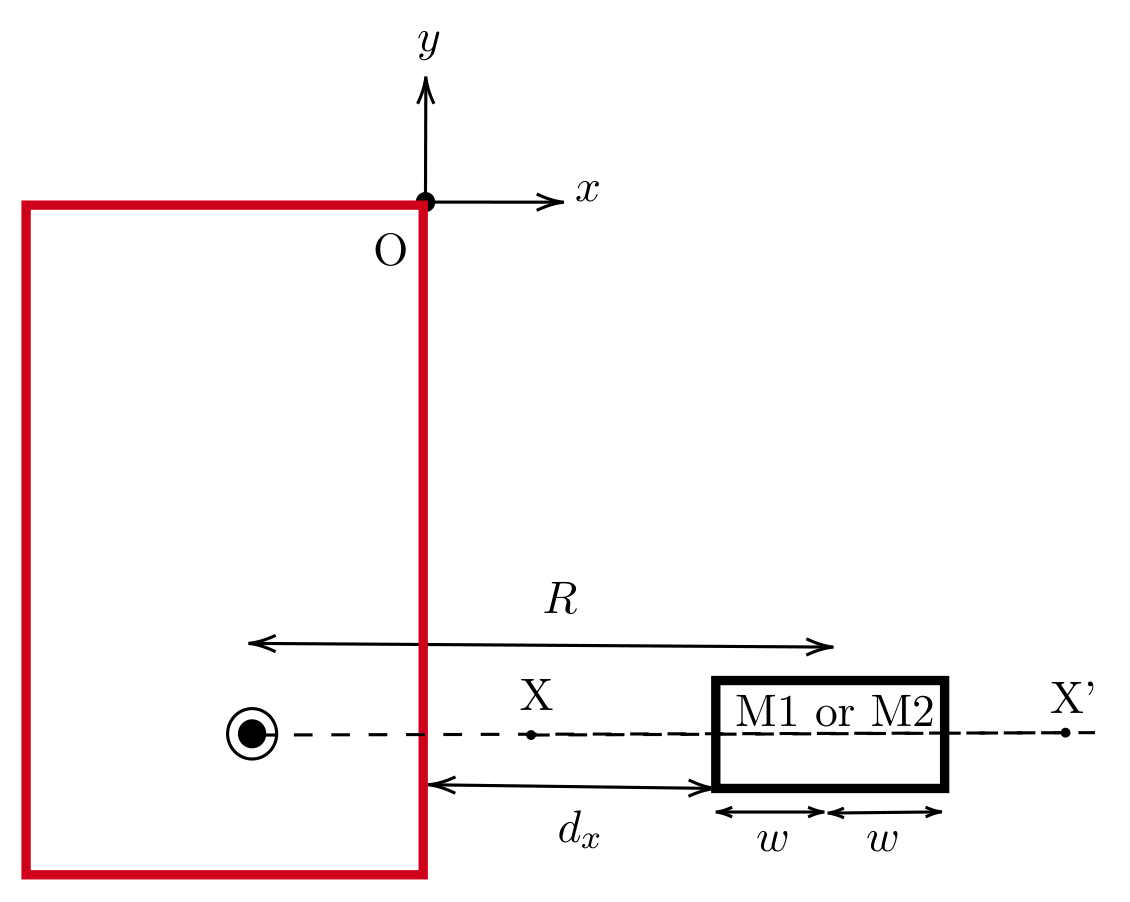
i. [5 marks] For the case of $R\gg w$ , obtain expressions for the net magnetic field $B$ at the magnetometer due to M1 and M2 in terms of $R,w,P'$ , and other constants. You may assume that each individual magnet can be modelled as a pair of magnetic monopoles separated by a distance $w$ .

ii. [10 marks] One set of Vanya’s data is presented in the table below.

$d_x$ (cm)	$B_x$ ( $\mu$ T)	$d_x$ (cm)	$B_x$ ( $\mu$ T)
2.1	-1359	3.1	-646
2.3	-1168	3.3	-563
2.5	-1001	3.5	-493
2.7	-855	3.7	-447
2.9	-743	3.9	-398

Plot a suitable linear graph to analyze the data, and from the graph, identify whether the data belongs to M1 or M2. Justify your answer. From the same linear plot (or a different one), calculate $P'$ of the individual magnets used in constructing the magnetic set.

Решение

(a) Solution: Let us understand this by an example when conducting a horizontal scan with the magnet in orientation IV, the behavior of the $B_x$ component of the magnetic field varies as follows:

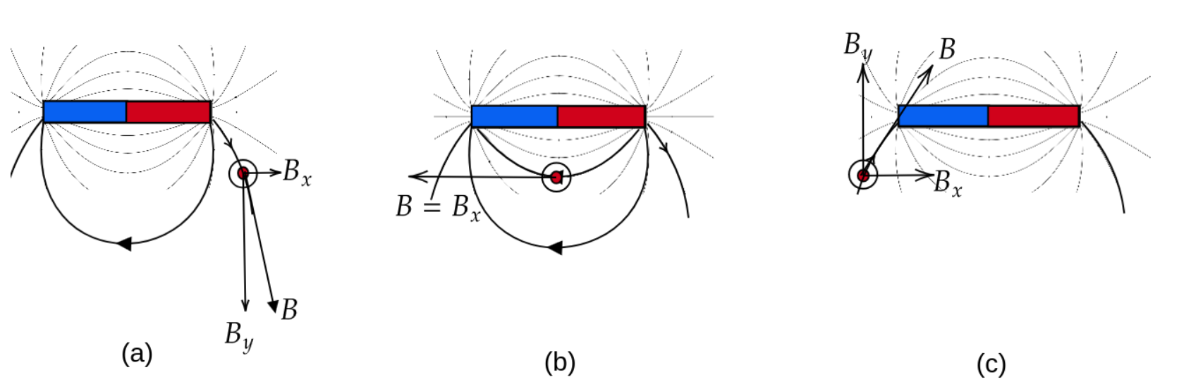
All three original horizontal orientation-IV field-line diagrams, magnet/sensor/field-vector components and a/b/c labels.

The magnetometer is to the right of the magnet. The magnetic field lines indicate that $B_x$ is directed to the right, corresponding to a positive $B_x$ value (see fig. (a)).
As the magnet moves rightward toward the center of the magnet, $B_x$ decreases, passing through zero (indicating a change in direction).
When the magnetometer aligns with the center of the magnet, $B_x$ reaches its maximum negative value, pointing entirely to the left (see fig. (b)).
$B_x$ increases from its negative peak, crossing zero again.
With the magnetometer to the left of the magnet, $B_x$ is directed to the right once more, yielding a positive value (see fig. (c)).

This progression results in a $B_x$ vs. $r_x$ plot that starts with a positive value at (a), descends to a negative peak at (b), and returns to a positive value at (c). This is qualitatively depicted in the figure below.

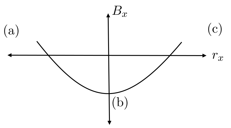
Complete native orientation-IV qualitative Bx-rx curve/axes/arrows and a/b/c labels.

Orientation III will produce a graph that is the exact opposite of the previous one, with the signs of $B_x$ reversed, as the dipole vector is now aligned in the $-x$ direction.

Let us consider another example with Orientation I, as shown in the figure below.

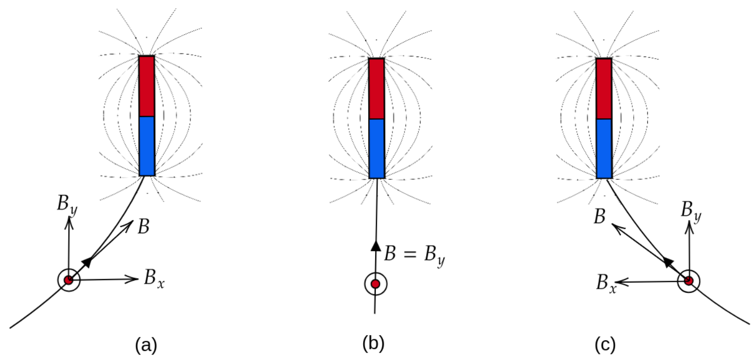
All three original orientation-I field-line diagrams, magnet/sensor/B/Bx/By arrows and a/b/c labels.

In this case, $B_x$ is positive when the magnet is to the right of the magnetometer (a), zero when the center of the magnet aligns with the magnetometer (b), and negative (pointing left) when the magnet is to the left of the magnetometer (c). This is qualitatively depicted in the figure below.

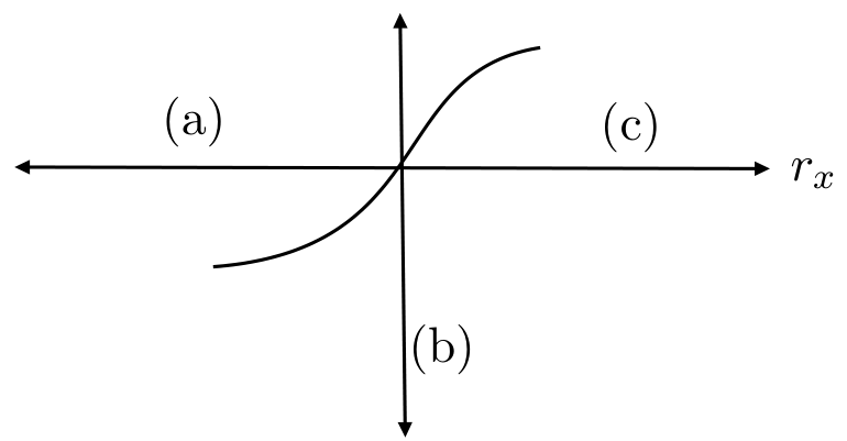
Complete native orientation-I qualitative S-curve/r_x/axes/arrows and a/b/c labels.

Orientation II will be just the opposite of Orientation I.

Similarly, we can analyze the vertical scan graphs. In this case, $B_x$ will vary like $B_y$ in the horizontal scan. Therefore, you can change the axis symbols in the diagrams above to reflect this adjustment for the vertical scan.

Considering the above analysis, we can summarize the results in the table below.

Scan	Plot	Orientation
Horizontal scan	A	II
Horizontal scan	B	III
Vertical scan	C	I
Vertical scan	D	IV

Magnetometer coordinates:

The magnet’s centre aligns with the magnetometer when the graph B peaks during the horizontal scan. This happens at $r_x=-2\ \mathrm{cm}$ . At this position, the magnet’s centre is located at -2 cm, which corresponds to the $x$ -coordinate of the magnetometer. Similarly, the vertical scan provides the $y$ -coordinate of the magnetometer, which is found to be -1 cm.

Coordinates of magnetometer are: $(-2,-1)\ \mathrm{cm}$

(b)i. Solution: Derivation for M1:

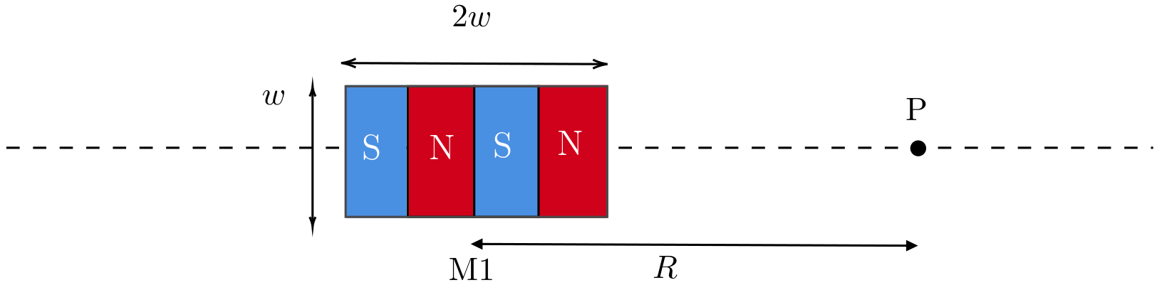
Entire M1 pole diagram/2w/w/R/P labels and dotted central axis.

For M1, if we consider the pole strength to be $m$ for each pole, the magnetic field at point $P$ , which is at a distance $r$ from the center of the magnet, can be expressed as:

B=\frac{\mu_0}{4\pi}\left(-\frac m{(R+w)^2}+\frac m{R^2}-\frac m{R^2}+\frac m{(R-w)^2}\right)

B=\frac{\mu_0m}{4\pi R^2}\left(-\left(1+\frac wR\right)^{-2}+\left(1-\frac wR\right)^{-2}\right)

We can use the approximation $\frac wR\ll1$ and simplify the expression up to the third order term in $w/R$ :

B\approx-\frac{\mu_0m}{4\pi R^2}\left(\left(1-\frac{2w}{R}+\frac{3w^2}{R^2}\right)-\left(1+\frac{2w}{R}+\frac{3w^2}{R^2}\right)\right)\qquad(4.1)

\boxed{B=4\frac{\mu_0P'}{4\pi R^3}}\qquad(4.2)

where $P'=mw$ is the dipole moment of the individual magnets in M1.

Similarly for M2:

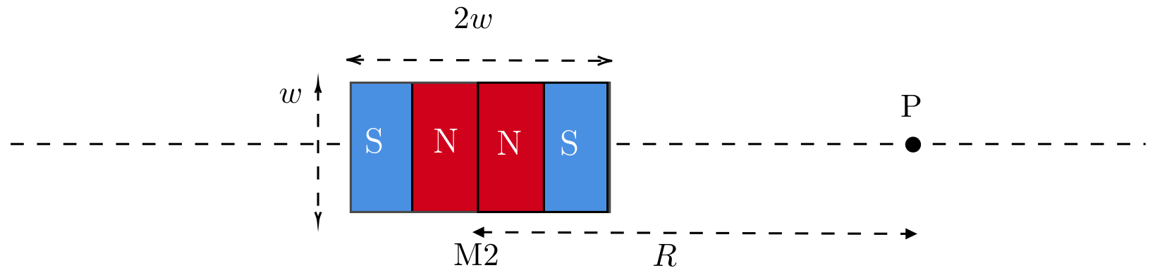
Entire M2 pole diagram/2w/w/R/P labels and dotted central axis.

the magnetic field at P due to the individual poles can be written as:

B=\frac{\mu_0}{4\pi}\left(-\frac m{(R+w)^2}+\frac m{R^2}+\frac m{R^2}-\frac m{(R-w)^2}\right)

B=\frac{\mu_0m}{4\pi R^2}\left(-\left(1+\frac wR\right)^{-2}+2-\left(1-\frac wR\right)^{-2}\right)

Keeping only up to the $(w/R)^3$ terms:

B=\frac{\mu_0m}{4\pi R^2}\left(-\left(1-\frac{2w}{R}+\frac{3w^2}{R^2}\right)+2-\left(1+\frac{2w}{R}+\frac{3w^2}{R^2}\right)\right)\qquad(4.3)

\boxed{B=-6\frac{\mu_0P'w}{4\pi R^4}}\qquad(4.4)

where $P'$ is the dipole moment of the individual magnets used in $M_2$ .

(b)ii. Solution: Linearizing the data for M2:

If we take the logarithm of Eqs. (4.2) and (4.4), we obtain:

\ln|B|=3\ln R+\ln\left(\frac{4P'\mu_0}{4\pi}\right),\qquad(4.5)

\ln|B|=4\ln R+\ln\left(\frac{6P'w\mu_0}{4\pi}\right).\qquad(4.6)

Thus, a plot of $\ln|B|$ vs. $\ln R$ will be linear, and the slope of this plot will indicate whether the dataset corresponds to M1 or M2.

Updated dataset after adjusting the lengths

$R=\lvert x_0\rvert+d_x+w$ (cm)	$\lvert B\rvert$ ( $\mu$ T)	$\ln R$	$\ln B$
5.1	1359	-2.975	-6.60
5.3	1168	-2.937	-6.75
5.5	1001	-2.900	-6.91
5.7	855	-2.864	-7.06
5.9	743	-2.830	-7.20
6.1	646	-2.797	-7.34
6.3	563	-2.764	-7.48
6.5	493	-2.733	-7.62
6.7	447	-2.703	-7.71
6.9	398	-2.673	-7.83

The graph is plotted on the Pg. 19.

The slope of the graph = 4.08.

Which indicates that the dataset corresponds to M2.

The intercept of the graph is $\ln\left(\frac{6P'w\mu_0}{4\pi}\right)=18.74\Rightarrow\boxed{P'=1.21\ \mathrm{A\cdot m^2}}$ .

The acceptable range of $P'$ is: $1.00-2.00\ \mathrm{A\cdot m^2}$ .

Whole native handwritten magnetic-data graph with original answer-page heading/grid/all ten points/axis labels/scales/negative slope and intercept annotations.

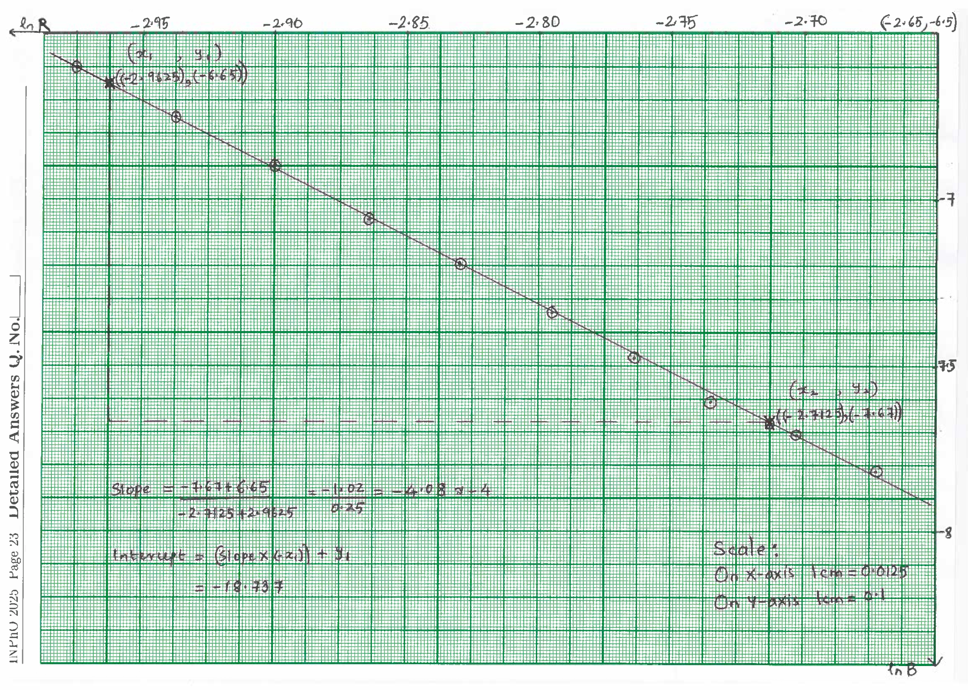
Source note: The boxed M1 derivation says distance $r$ while its diagram and formulas use $R$ . Both approximation paragraphs say third-order terms, although the displayed expansions stop at quadratic terms. Equations (4.5)–(4.6) print positive $3\ln R$ and $4\ln R$ ; the printed table and native handwritten graph show a decreasing trend. The typed slope is positive 4.08 and the typed intercept is positive 18.74, while the handwriting records a slope of approximately -4.08 (approximately -4) and an intercept of approximately -18.737. The table header is $\ln B$ despite negative measured fields; its numerical logarithms are retained. These discrepancies remain visible; the native graph is reproduced whole, rotated for reading without redrawing or changing annotations.

Native source end

END OF THE QUESTION PAPER

The key also ends with this native wording on page24. Key page20 is blank apart from running page and roll-number furniture.

Оригинал в Архива: INPhO2025-Question.pdf · официални решения: INPhO2025-Solution-20250219.pdf