Съдържание

Условие a)b)c)General examination instructions Решение

IOAA 2014, Анализ на данни · окончателна тема — Задача 1. Black Hole in Milky Way

Оригинал на условието (изображение)Съобщи за грешка

Всички материали от IOAA 2014

8th IOAA · Final data analysis paper

Внимание: Бележка към темата

The final paper is preserved in six photographed sheets. Its three whole problems differ from the preliminary solution booklet: Black Hole is renumbered, Thermodynamic test is separate, and the observer problem replaces seven Big Dipper stars with four Mizar-system stars and adds uncertainty estimates. Applicable key material is distinguished from variant comparisons; absent final-key portions and the missing orbit-plot annex are explicit.

Условие

By observational facts, the scientists admit presence of a black-hole at the center of Milky Way.
At the center of Milky Way, a hypothetical black-hole (Sagittarius A*) is located. A star S* is orbiting the black-hole SA*.

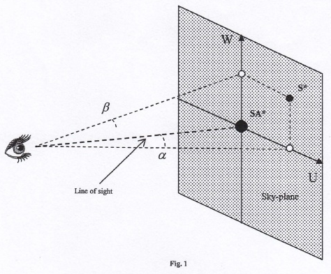
In the table 1 the following data is presented: the date and the angular position coordinates $(\alpha;\beta)$ of the star S* at different moments of the observation. The coordinates represent the angular distances of the projection of the star S* in the coordinates system (U, W), centered on the SA* (see figure 1).
An angular distance of $\varphi=1\,\text{arcsec}$ corresponds to linear distance in the plane of the sky $d=41$ light days, therefore to a scale

S_0=\frac d\varphi=41\,\frac{\text{light day}}{\text{arcsec}}.

	Date (year)	$\alpha$ (arcsec)	$\beta$ (arcsec)
1	1995.222	0.117	-0.166
2	1997.526	0.097	-0.189
3	1998.326	0.087	-0.192
4	1999.041	0.077	-0.193
5	2000.414	0.052	-0.183
6	2001.169	0.036	-0.167
7	2002.831	-0.000	-0.120
8	2003.584	-0.016	-0.083
9	2004.165	-0.026	-0.041
10	2004.585	-0.017	0.008
11	2004.655	-0.004	0.014
12	2004.734	0.008	0.017
13	2004.839	0.021	0.012
14	2004.936	0.037	0.009
15	2005.503	0.072	-0.024
16	2006.041	0.088	-0.050
17	2007.060	0.108	-0.091

Fig. 1. Angular coordinates in the sky plane.

By using the information provided your tasks are:

a)

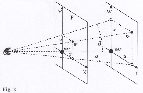
Plot the projection of the trajectory of the star S* in the plane P (see figure 2). This plane is close to the observer. In this plane, $\varphi=1\,\text{arcsec}$ corresponds to a linear distance $d_0=1200\,\mathrm{mm}$ therefore the scale is

S=\frac{d_0}{\varphi}=1200\,\frac{\mathrm{mm}}{\text{arcsec}}.

You have to use the millimeter graph paper, carbon copy sheet of paper and the transparent sheets for an accurate plot.

Fig. 2. Projection onto the drawing plane P.

b)

By using the plot prove that the line of sight is normal to the actual plane of the orbit

c)

Using your plot find out following elements of the real orbit of star S* around the black hole SA*:

I. $a$ – semi-major axis (in light days units); $b$ – small semi-minor axis (in light days units); $e$ – eccentricity;
II. $r_{\min}$ – the minimum distance between S* and SA* (in light days units); $r_{\max}$ – the maximum distance between S* and SA* (in light days units);
III. The distance from the observer to the S*;
IV. the orbiting period of star S* around SA* (obtain the best possible result by taking as many measurements as possible and by taking their arithmetic mean);
V. the total mass of the system “SA* – S*”.

Presenting the intermediate and final data in tables is recommended for an accurate evaluation.

G=6.67\cdot10^{-11}\,\mathrm{N\,m^2\,kg^{-2}}.

General examination instructions

In your folder you will find out the following: a) Answer sheets
b) Draft sheets
c) The envelope with the subjects in English and the translated version of them in your mother tongue;
The solutions of the problems will be written down only on the answer sheets you receive on your desk. PLEASE WRITE ONLY ON THE PRINTED SIDE OF THE PAPER SHEET. DON'T USE THE REVERSE SIDE. The evaluator will not take into account what is written on the reverse of the answer sheet.
The draft sheets is for your own use to try calculation, write some numbers etc. BEWARE: These papers are not taken into account in evaluation, at the end of the test they will be collected separately. Everything you consider as part of the solutions have to be written on the answer sheets.
Each problem have to be started on a new distinct answer sheet.
On each answer sheet please fill in the designated boxes as follows: a) In PROBLEM NO. box write down only the number of the problem: i.e. 1–3. Each sheet containing the solutions of a certain problem, should have in the box the number of the problem;
b) In Student ID – fill in your ID you will find on your envelope, consisted of 3 letters and 2 digits.
c) In page no. box you will fill in the number of page, starting from 1. We advise you to fill this boxes after you finish the test
We don't understand your language, but the mathematic language is universal, so use as more relationships as you think that your solution will be better understand by the evaluator. If you want to explain in words we kindly ask you to use short English propositions.
Use the pen you find out on the desk. It is advisable to use a pencil for the sketches.
At the end of the test: a) Don't forget to put in order your papers;
b) Put the answer sheets in the folder 1. Please verify that all the pages contain your ID, correct numbering of the problems and all pages are in the right order and numbered. This is an advantage of ease of understanding your solutions.
c) Verify with the assistant the correct number of answer sheets used fill in this number on the cover of the folder and sign.
d) Put the draft papers in the designated folder. Put the test papers back in the envelope.
e) Go to swim

GOOD LUCK!

Решение

Внимание: Непълно решение

The available key is labelled preliminary Problem 2. It matches the final data and requests, but does not give the requested observer distance in c(III), and its referenced orbit-plot annex is absent from the checked 39-page PDF and year inventory.

The archived booklet labels this problem 2; it is problem 1 on the final photographed paper. Its marking scheme is a) 15 points, b) 10 points and c) 25 points, with 5 points for each of I–V. The calculations below retain the printed numbers and discrepancies.

Detailed solution

Usually the plane of apparent orbit (sky plane) is different from the plane of the relative orbit due to the angle between the two planes ( $i=0$ ).

Original comparison of real and apparent orbital planes.

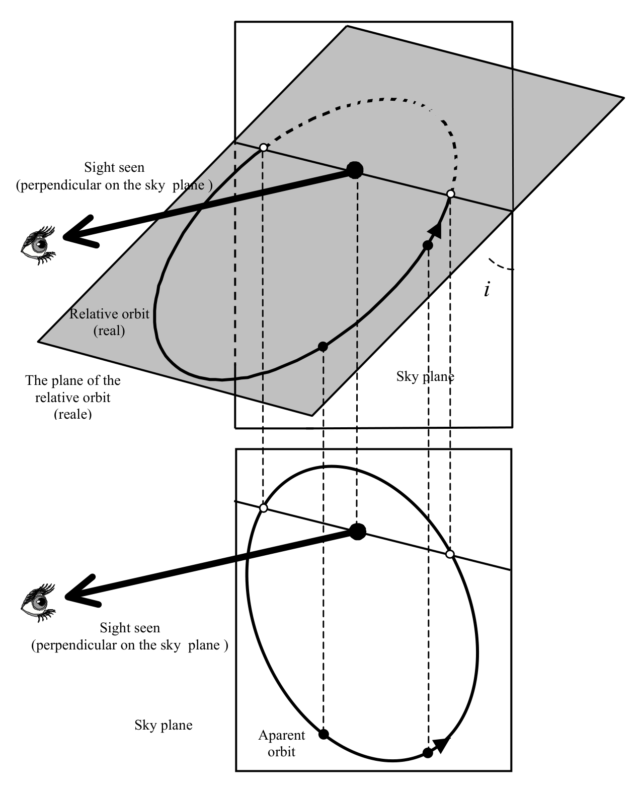
In the case of the problem the sky plane and the plane of the relative orbit are the same ( $i=0$ ). See the figure.

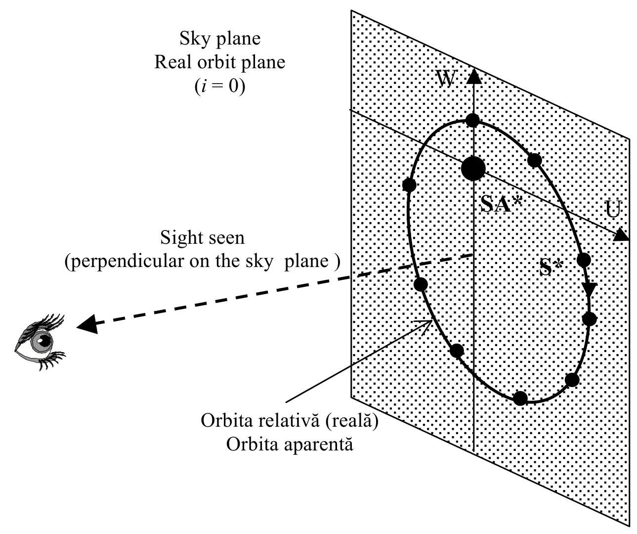
Original coincident sky and orbit planes, i=0.

The linear position coordinates $(u,w)$ of the projection of the star S* in the sky plane with the coordinate axes (U, W), having the origin in Sagittarius A*, expressed in light-days are given in table 1. For an angular distance $\varphi=1\,\text{arcsec}$ correspond in sky plane the linear distance $d=41$ light day.

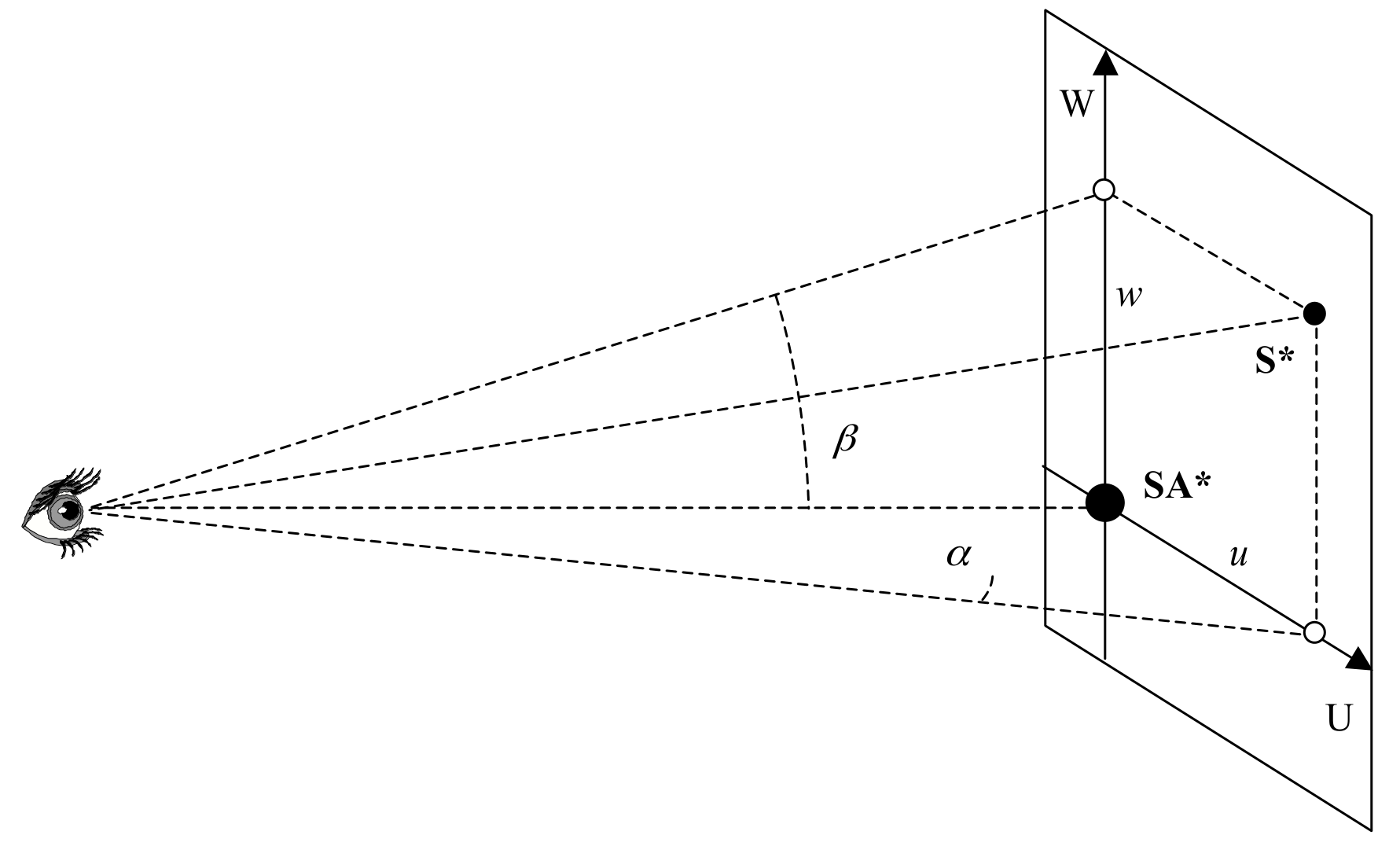
Source note: the first sentence prints $i=0$ while describing different planes; the later sentence also prints $i=0$ for coincident planes. Both are retained.

Coordinate tables

	Date (year)	$\alpha$ (arcsec)	u (ld)	$\beta$ (arcsec)	w (ld)
1	1995.222	0.117	4.797	-0.166	-6.806
2	1997.526	0.097	3.977	-0.189	-7.749
3	1998.326	0.087	3.567	-0.192	-7.872
4	1999.041	0.077	3.157	-0.193	-7.913
5	2000.414	0.052	2.132	-0.183	-7.503
6	2001.169	0.036	1.476	-0.167	-6.847
7	2002.831	-0.000	0.000	-0.120	-4.920
8	2003.584	-0.016	-0.656	-0.083	-3.403
9	2004.165	-0.026	-1.066	-0.041	-1.681
10	2004.585	-0.017	-0.697	0.008	0.328
11	2004.655	-0.004	-0.164	0.014	0.574
12	2004.734	0.008	0.328	0.017	0.697
13	2004.839	0.021	0.861	0.012	0.492
14	2004.936	0.037	1.517	0.009	0.369
15	2005.503	0.072	2.952	-0.024	-0.984
16	2006.041	0.088	3.608	-0.050	-2.050
17	2007.060	0.108	4.428	-0.091	-3.731

To represent the image of the relative orbit of star S* in a plane parallel with the sky plane we use a scale of $S=1200\,\mathrm{mm/arcsec}$ , and for conversion we use $x=\alpha S$ and $y=\beta S$ , see figure 3. These coordinates of the image of the star S* relative to the origin of the axes – the image of Sagittarius A* – are given in the below table 3.

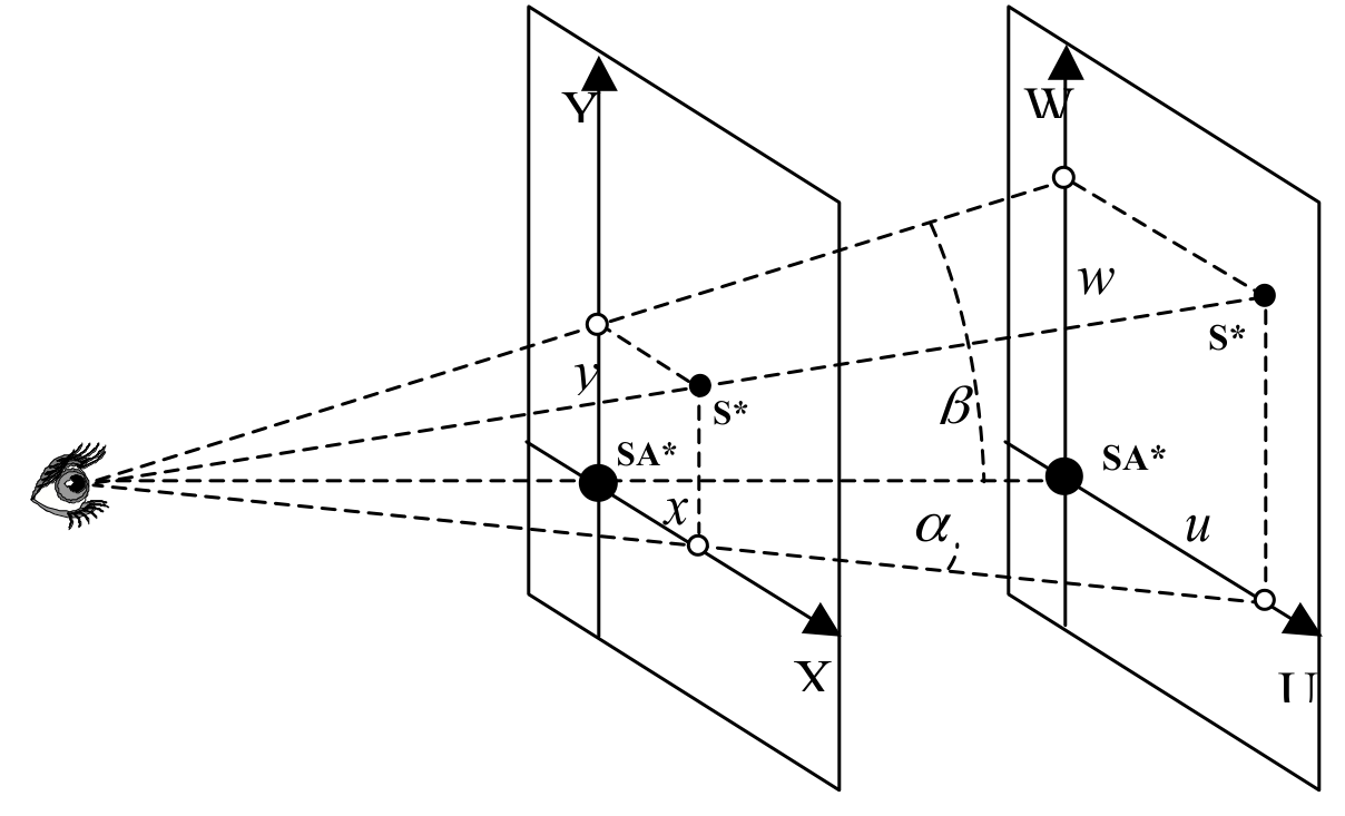
Original mapping from sky plane to drawing plane.

Table 2. The coordinates in scaled plane

	Date (year)	$\alpha$ (arcsec)	x (mm)	$\beta$ (arcsec)	y (mm)
1	1995.222	0.117	140.4	-0.166	-199.2
2	1997.526	0.097	116.4	-0.189	-226.8
3	1998.326	0.087	104.4	-0.192	-230.4
4	1999.041	0.077	92.4	-0.193	-231.6
5	2000.414	0.052	62.4	-0.183	-219.6
6	2001.169	0.036	43.2	-0.167	-200.4
7	2002.831	-0.000	0.0	-0.120	-144.0
8	2003.584	-0.016	-20.0	-0.083	-100.0
9	2004.165	-0.026	-32.0	-0.041	-50.0
10	2004.585	-0.017	-20.4	0.008	9.6
11	2004.655	-0.004	-4.8	0.014	16.8
12	2004.734	0.008	9.6	0.017	20.4
13	2004.839	0.021	25.2	0.012	14.4
14	2004.936	0.037	44.4	0.009	10.8
15	2005.503	0.072	86.4	-0.024	-28.8
16	2006.041	0.088	106.0	-0.050	-60.0
17	2007.060	0.108	130.0	-0.091	-110.0

The following pictures represents the plot of the values in the table 2, and the measurements which have to be done in order to find out the required data.

Source note: the numerical table is reproduced as printed, including rounded values that do not exactly equal the stated angular coordinate times 1200. The referenced completed orbit plot is not present in the available file.

Numeric processing — a)

From the measurements done on paper system (X, Y):

a_{maesured}\approx135\,\mathrm{mm};\ b_{mesured}\approx66\,\mathrm{mm};\ d_{\min}=17\,\mathrm{mm},

Corresponding to the numeric scale:

a_{mesured}=\varphi_a\cdot S;\ b_{mesured}=\varphi_b\cdot S;\ d_{\min}{}^{mes}=\varphi_{\min}\cdot S,

\varphi_a=0.1125\ \mathrm{arcsec};

\varphi_b=0.055\ \mathrm{arcsec};

\varphi_{d\min}=0{,}01416\ \mathrm{arcsec};

1\ \mathrm{arcsec}\ \ldots\ldots\ldots\ldots\ 41\ \text{light day};

\varphi_a=0.1125\ \mathrm{arcsec}\ \ldots\ldots\ldots\ a;

\varphi_b=0.055\ \mathrm{arcsec}\ \ldots\ldots\ldots\ b;

\varphi_{d\min}=0{,}014666\ \mathrm{arcsec}\ \ldots\ldots\ldots\ r_{\min};

a=\frac{0.1125\ \mathrm{arcsec}\cdot41\ \text{light days}}{1\ \mathrm{arcsec}};\ a=4.6125\ \text{light days},

b=\frac{0.055\ \mathrm{arcsec}\cdot41\ \text{light days}}{1\ \mathrm{arcsec}};\ b=2.255\ \text{light days},

r_{\min}=\frac{0{,}0146\ \mathrm{arcsec}\cdot41\ \text{light days}}{1\ \mathrm{arcsec}}=0{,}5986\ \text{light days};

c=\sqrt{a^2-b^2}\approx4{,}0236\ \text{light days};

r_{\min}=a-c=0{,}5889\ \text{light days};\ r_{\max}=a+c=8{,}6361\ \text{light days};

e=\sqrt{1-\frac{b^2}{a^2}}\approx0.87,

Numeric processing — b)

$S_{\text{elipsa}}=28560\,\mathrm{mm^2}$ ; See Anex

T\longleftrightarrow S_{\text{elipsa}},\quad\Delta t\longleftrightarrow\Delta S,\qquad T=\frac{S_{\text{elipsa}}}{\Delta S}\Delta t.

The printed step-by-step area and period calculations are tabulated below. For every row, $\Delta S=\ell w/2+\text{correction}$ , $\Delta t=t_{\rm end}-t_{\rm start}$ , and $T=28560\,\Delta t/\Delta S$ . Dates are in years and areas in mm². All intermediate and final printed values are retained.

Displacement	Start year	End year	$\ell$ (mm)	w (mm)	Correction (mm²)	$\Delta S$ (mm²)	$\Delta t$ (years)	T (years)
1→2	1995.222	1997.526	252	34	86	4370	2.304	15.057
2→3	1997.526	1998.326	252	12	20	1532	0.800	14.913
3→4	1998.326	1999.041	250	11	26	1400	0.715	14.586
4→5	1999.041	2000.414	244	22	30	2714	1.373	14.448
5→6	2000.414	2001.169	220	13	5	1435	0.755	15.026
6→7	2001.169	2002.831	203	30	120	3165	1.662	14.997
7→8	2002.831	2003.584	143	20	5	1435	0.753	14.986
8→9	2003.584	2004.165	100	22	7	1107	0.581	14.989
9→10	2004.165	2004.585	60	20	200	800	0.420	14.994
10→11	2004.585	2004.655	20	13	5	135	0.070	14.808
11→12	2004.655	2004.734	22	13	4	147	0.077	14.960
12→13	2004.734	2004.839	30	13	4	200	0.105	14.994
13→14	2004.839	2004.936	41	9	0	185	0.097	14.974
14→15	2004.936	2005.503	90	22	90	1080	0.567	14.994
15→16	2005.503	2006.041	120	17	5	1025	0.538	14.990
16→17	2006.041	2007.060	168	23	10	1942	1.019	14.985
17→1	2007.060	not stated (next cycle)	240	43	300	5460	2,867	14.996

\overline T=14.923\,\text{years};\qquad T\approx15\,\text{years}.

Source notes: for 17→1 the printed area expression writes $240\,\mathrm{mm}\times43\,\mathrm m/2+300\,\mathrm{mm^2}=5460\,\mathrm{mm^2}$ ; its metre unit is inconsistent with the other rows. The 11→12 time difference is printed 0.077 despite the listed dates. The mean and all individual periods are the source values. The “Anex” is absent from the available file.

Numeric processing — c)

By using the III rd Kepler's law:

T^2=\frac{4\pi^2}{K(M_{\rm SA*}+M_{\rm S*})}a^3;\qquad M_{\rm SA*}+M_{\rm S*}=\frac{4\pi^2a^3}{KT^2};

a=4.6125\,\text{light days};\quad T\approx15\,\text{years};\quad K=6{,}67\cdot10^{-11}\,\mathrm{N\,m^2\,kg^{-2}};

1\,\mathrm{ld}\approx2{,}6\cdot10^{13}\,\mathrm m;\quad1\,\text{years}\approx3{,}1\cdot10^7\,\mathrm s;\quad4\pi^2\approx40;

(2{,}6)^3\approx17{,}6;\qquad(4.6125)^3\approx10^2;

M_{\rm SA*}+M_{\rm S*}=\frac{40\cdot10^2\cdot17{,}6\cdot10^{39}}{6{,}67\cdot10^{-11}\cdot225\cdot10^{15}}\,\mathrm{kg}\approx4{,}6\cdot10^{36}\,\mathrm{kg};

M_{\text{Sun}}\approx1{,}8\cdot10^{30}\,\mathrm{kg};\qquad M_{\rm SA*}+M_{\rm S*}\approx2{,}5\cdot10^6M_{\text{Sun}};

M_{\rm S*}\ll M_{\rm SA*};\qquad M_{\rm SA*}\approx2{,}5\cdot10^6M_{\text{Sun}}.

The printed approximations, gravitational-constant symbol K and solar mass are retained.

Оригинал в Архива: ioaa11.jpg · официални решения: DA_Solution.pdf · допълнителни данни: ioaa12.jpg · допълнителни данни: ioaa13.jpg · допълнителни данни: ioaa14.jpg · допълнителни данни: ioaa15.jpg · допълнителни данни: ioaa16.jpg