Съдържание

IOAA 2016, Анализ на данни — Задача 1. Binary Pulsar

Оригинал на условието (PDF)Съобщи за грешка

Всички материали от IOAA 2016

Data Analysis Examination · 50 т.

Условие

Through systematic searches during the past decades, astronomers have found a large number of millisecond pulsars (spin period $< 10\ \mathrm{ms}$ ). Majority of these pulsars are found in binaries, with nearly circular orbits.

For a pulsar in a binary orbit, the measured pulsar spin period ( $P$ ) and the measured line-of-sight acceleration ( $a$ ) both vary systematically due to orbital motion. For circular orbits, this variation can be described mathematically in terms of orbital phase $\phi$ ( $0 \le \phi \le 2\pi$ ) as,

P(\phi) = P_0 + P_{\mathrm{t}} \cos\phi \qquad \text{where } P_t = \frac{2\pi P_0 r}{c P_{\mathrm{B}}}

a(\phi) = -a_{\mathrm{t}} \sin\phi \qquad \text{where } a_{\mathrm{t}} = \frac{4\pi^2 r}{P_{\mathrm{B}}^2}

where $P_{\mathrm{B}}$ is the orbital period of the binary, $P_0$ is the intrinsic spin period of the pulsar and $r$ is the radius of the orbit.

The following table gives one such set of measurements of $P$ and $a$ at different heliocentric epochs, $T$ , expressed in truncated Modified Julian Days (tMJD), i.e. number of days since MJD = 2,440,000.

No.	T (tMJD)	P (μs)	a (m s $^{-2}$ )
1	5740.654	7587.8889	- 0.92 ± 0.08
2	5740.703	7587.8334	- 0.24 ± 0.08
3	5746.100	7588.4100	- 1.68 ± 0.04
4	5746.675	7588.5810	+ 1.67 ± 0.06
5	5981.811	7587.8836	+ 0.72 ± 0.06
6	5983.932	7587.8552	- 0.44 ± 0.08
7	6005.893	7589.1029	+ 0.52 ± 0.08
8	6040.857	7589.1350	+ 0.00 ± 0.04
9	6335.904	7589.1358	+ 0.00 ± 0.02

By plotting $a(\phi)$ as a function of $P(\phi)$ , we can obtain a parametric curve. As evident from the relations above, this curve in the period-acceleration plane is an ellipse.

In this problem, we estimate the intrinsic spin period, $P_0$ , the orbital period, $P_{\mathrm{B}}$ , and the orbital radius, $r$ , by an analysis of this data set, assuming a circular orbit.

(D1.1) Plot the data, including error bars, in the period-acceleration plane (mark your graph as “D1.1”). [7 т.]

(D1.2) Draw an ellipse that appears to be a best fit to the data (on the same graph “D1.1”). [2 т.]

(D1.3) From the plot, estimate $P_0$ , $P_{\mathrm{t}}$ and $a_{\mathrm{t}}$ , including error margins. [7 т.]

(D1.4) Write expressions for $P_{\mathrm{B}}$ and $r$ in terms of $P_0$ , $P_{\mathrm{t}}$ , $a_{\mathrm{t}}$ . [4 т.]

(D1.5) Calculate approximate value of $P_{\mathrm{B}}$ and $r$ based on your estimations made in (D1.3), including error margins. [6 т.]

(D1.6) Calculate orbital phase, $\phi$ , corresponding to the epochs of the following five observations in the above table: data rows 1, 4, 6, 8, 9. [4 т.]

(D1.7) Refine the estimate of the orbital period, $P_{\mathrm{B}}$ , using the results in part (D1.6) in the following way:

(D1.7a) First determine the initial epoch, $T_0$ , which corresponds to the nearest epoch of zero orbital phase before the first observation. [2 т.]

(D1.7b) The expected time, $T_{\mathrm{calc}}$ , of the estimated orbital phase angle of each observation is given by,

T_{\mathrm{calc}} = T_0 + \left(n + \frac{\phi}{360^{\circ}}\right) P_{\mathrm{B}},

where $n$ is the number of full cycle of orbital phases that may have elapsed between $T_0$ and $T$ (or $T_{\mathrm{calc}}$ ). Estimate $n$ and $T_{\mathrm{calc}}$ for each of the five observations in part (D1.6). Note down difference $T_{\mathrm{O-C}}$ between observed $T$ and $T_{\mathrm{calc}}$ . Enter these calculations in the table given in the Summary Answersheet. [7 т.]

(D1.7c) Plot $T_{\mathrm{O-C}}$ against $n$ (mark your graph as “D1.7”). [4 т.]

(D1.7d) Determine the refined values of the initial epoch, $T_{0,\mathrm{r}}$ , and the orbital period, $P_{\mathrm{B,r}}$ . [7 т.]

Отговори

Решение

(D1.1)

Graph Number : D1.1

Plot uses more than 50% of graph paper: 0.5
Axes labels ( $P$ and $a$ ): 0.5
Dimensions of axes: 0.5
Ticks and values on axes (or scale written explicitly): 0.5
Points correctly plotted:

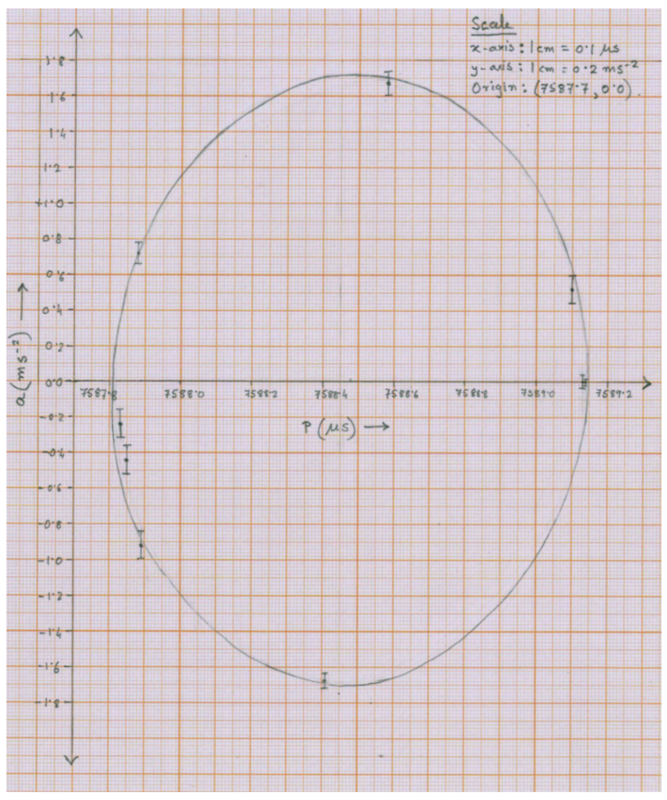
Hand-drawn graph D1.1 on graph paper: acceleration a (m s⁻²) from −1.8 to 1.8 against period P (μs) from 7587.8 to 7589.2, nine data points with error bars and a fitted ellipse; scale note: x-axis 1 cm = 0.1 μs, y-axis 1 cm = 0.2 m s⁻², origin (7587.7, 0.0).

Points plotted	9	8	7	6	5	$< 5$
Marks given	4.0	3.5	3.0	2.0	1.0	0

Correctness of points: deduction of 0.5 for each wrong point.

Errorbars on points (at least 5): 1.0

(D1.2)

See above

Elliptical curve with visual best fit: 1.0
Curve symmetric about $a = 0$ line: 0.5
Curve symmetric about some value of $P$ ( $P \approx 7588.48$ ): 0.5

(D1.3)

Values are determined from lengths of axes of ellipse and mid-point of $P$ -axis.

Error margins may be determined by estimating extreme ellipses covering the points with errorbars. Any reasonable method of estimating error margins will be accepted.

$2P_{\mathrm{t}} = (1.34 \pm 0.04)\ \mathrm{\mu s}$ [ $(13.4 \pm 0.4)\ \mathrm{cm}$ on graph]

$\boxed{P_{\mathrm{t}} = (0.67 \pm 0.02)\ \mathrm{\mu s}}$ [2.0]

$\boxed{P_0 = (7588.48 \pm 0.02)\ \mathrm{\mu s}}$ [2.0]

$2a_{\mathrm{t}} = (3.42 \pm 0.12)\ \mathrm{m\,s^{-2}}$ [ $(17.1 \pm 0.6)\ \mathrm{cm}$ on graph] [3.0]

$\boxed{a_{\mathrm{t}} = (1.71 \pm 0.06)\ \mathrm{m\,s^{-2}}}$

Marking table:

Parameter	Half credit Minimum	Full credit Minimum	Full credit Maximum	Half credit Maximum
$P_{\mathrm{t}}$ (μs)	0.59	0.63	0.71	0.75
$\delta P_{\mathrm{t}}$ (μs)	0.01	0.02	0.04	0.05
$P_0$ (μs)	7588.38	7588.43	7588.53	7588.58
$\delta P_0$ (μs)	0.01	0.02	0.04	0.05
$a_{\mathrm{t}}$ (m s $^{-2}$ )	1.61	1.65	1.77	1.81
$\delta a_{\mathrm{t}}$ (m s $^{-2}$ )	0.04	0.05	0.07	0.08

Wrong values due to wrong/poor plot/fit in (D1.1) and (D1.2) WILL BE penalised.
Error estimation is based on graph drawing. Quoted values correspond to the envelope of possible ellipses drawn to include all points with errorbars. Any reasonable method to estimate error to be given credit.

(D1.4)

We can easily recover the orbital period ( $P_{\mathrm{B}}$ ) and the radius of the orbit ( $r$ ) in a circular orbit:

a_{\mathrm{t}} = \frac{4\pi^2}{P_{\mathrm{B}}^2} r

\therefore r = \frac{P_{\mathrm{B}}^2 a_{\mathrm{t}}}{4\pi^2}

[1.0]

P_{\mathrm{t}} = \frac{2\pi P_0}{P_{\mathrm{B}}} \times \frac{r}{c} = \frac{2\pi P_0}{P_{\mathrm{B}} c} \times \frac{P_{\mathrm{B}}^2 a_{\mathrm{t}}}{4\pi^2} = \frac{P_0 P_{\mathrm{B}} a_{\mathrm{t}}}{2\pi c}

\therefore \boxed{P_{\mathrm{B}} = \frac{P_{\mathrm{t}}}{P_0}\frac{2\pi c}{a_{\mathrm{t}}}}

[1.0]

r = \frac{a_{\mathrm{t}}}{4\pi^2}\left(\frac{P_{\mathrm{t}}}{P_0}\frac{2\pi c}{a_{\mathrm{t}}}\right)^2

[1.0]

\therefore \boxed{r = \left(\frac{P_{\mathrm{t}}}{P_0}\right)^2 \frac{c^2}{a_{\mathrm{t}}}}

[1.0]

Alternative algebraic routes accepted. Each of $P_{\mathrm{B}}$ and $r$ carry 2.0 marks.

(D1.5)

P_{\mathrm{B}} = \frac{P_{\mathrm{t}}}{P_0}\frac{2\pi c}{a_{\mathrm{t}}} = \frac{0.67}{7588.48} \times \frac{2\pi \times 2.998 \times 10^8}{1.71}\,\mathrm{s} = 96\,260\ \mathrm{s} = 1.125\,70\ \mathrm{d}

[1.0]

\Delta P_{\mathrm{B}} = P_{\mathrm{B}}\sqrt{\left(\frac{\Delta P_{\mathrm{t}}}{P_{\mathrm{t}}}\right)^2 + \left(\frac{\Delta P_0}{P_0}\right)^2 + \left(\frac{\Delta a_{\mathrm{t}}}{a_{\mathrm{t}}}\right)^2}

[1.0]

= 1.12570 \times \sqrt{\left(\frac{0.02}{0.67}\right)^2 + \left(\frac{0.02}{7588.48}\right)^2 + \left(\frac{0.06}{1.71}\right)^2}\,\mathrm{d} = 1.12570 \times 0.0461 \simeq 0.052\ \mathrm{d}

\therefore \boxed{P_{\mathrm{B}} = (1.13 \pm 0.05)\ \mathrm{d}}

[1.0]

r = \left(\frac{P_{\mathrm{t}}}{P_0}\right)^2 \frac{c^2}{a_{\mathrm{t}}} = \left(\frac{0.67}{7588.48}\right)^2 \times \frac{\left(2.998 \times 10^8\right)^2}{1.71}\,\mathrm{m}

\therefore r = 4.097\,39 \times 10^8\ \mathrm{m} = 2.738\,90 \times 10^{-3}\ \mathrm{AU}

[1.0]

\Delta r = r\sqrt{\left(\frac{2\Delta P_{\mathrm{t}}}{P_{\mathrm{t}}}\right)^2 + \left(\frac{2\Delta P_0}{P_0}\right)^2 + \left(\frac{\Delta a_{\mathrm{t}}}{a_{\mathrm{t}}}\right)^2}

[1.0]

= 2.738\,90 \times 10^{-3} \times \sqrt{\left(\frac{2 \times 0.02}{0.67}\right)^2 + \left(\frac{2 \times 0.02}{7588.48}\right)^2 + \left(\frac{0.06}{1.71}\right)^2}\,\mathrm{AU} = 2.738\,90 \times 10^{-3} \times 0.069\,25\ \mathrm{AU} \simeq 0.19 \times 10^{-3}\ \mathrm{AU}

\boxed{r = (2.74 \pm 0.19) \times 10^{-3}\ \mathrm{AU}}

[1.0]

Errors in $P_{\mathrm{B}}$ and $r$ can be also estimated as maximum possible (worst case) error. In such case, errors would be about 1.5 times the standard error calculated above ( $\delta P_{\mathrm{B}} = 0.07, \delta r = 0.25$ ).

(D1.6)

Using these newly determined orbital parameters, we can calculate the angular orbital phase for each data point, i.e., for each pair of acceleration and period measured ( $P$ , $a$ ).

\phi = \tan^{-1}\left(-\frac{a}{a_{\mathrm{t}}}\frac{P_{\mathrm{t}}}{P - P_0}\right)

Care has to be taken to choose the value of the phase from among $\phi, \pi \pm \phi, 2\pi - \phi$ , depending on the sign of $\cos\phi$ and $\sin\phi$ .

Sr. no.	$T$ (tMJD)	$P$ (μs)	$a$ (m s $^{-2}$ )	$\phi$
1	5740.654	7587.8889	−0.92	148.62°
4	5746.675	7588.5810	+1.67	278.77°
6	5983.932	7587.8552	−0.44	164.57°
8	6040.857	7589.1350	+0.00	0.00°
9	6335.904	7589.1358	+0.00	0.00°

Credit for each correct value: 1.0 for first three, 0.5 for last two.
Credit for $\pi \pm \phi$ or $2\pi - \phi$ is 0.5 per value.
All values wrong due to wrong expression for $\phi$ gets a maximum of 1.0 mark.
Values in radians accepted.

(D1.7a)

\frac{T_1 - T_0}{P_{\mathrm{B}}} = \frac{\phi_1}{2\pi} \Rightarrow T_0 = T_1 - \frac{\phi_1}{2\pi} P_{\mathrm{B}}

[1.0]

T_0 = 5740.654 - \frac{148.62^{\circ}}{360^{\circ}} \times 1.12570\ \mathrm{tMJD}

\boxed{T_0 = 5740.189\ \mathrm{tMJD}}

[1.0]

Tolerance: $\pm 0.002$ tMJD. Using $P_0$ instead of $P_{\mathrm{B}}$ gets zero.

(D1.7b)

T_{\mathrm{calc}} = T_0 + \left(n + \frac{\phi}{360^{\circ}}\right) P_{\mathrm{B}}

where $n =$ Integer part of $[(T - T_0)/P_{\mathrm{B}}]$ .

Sr. No.	$T$ (tMJD)	$\phi$	$n$	$T_{\mathrm{calc}}$ (MJD)	$T_{\mathrm{O-C}}$ (days)
1	5740.654	148.62°	0	5740.654	0.000
4	5746.675	278.77°	5	5746.689	−0.014
6	5983.932	164.57°	216	5983.855	0.077
8	6040.857	0.00°	267	6040.751	0.106
9	6335.904	0.00°	529	6335.684	0.220

Deduction for each wrong/missing value of $n$ , $T_{\mathrm{calc}}$ and $T_{\mathrm{O-C}}$ : 0.5

No double penalty in one row.

(D1.7c)

Graph Number : D1.7

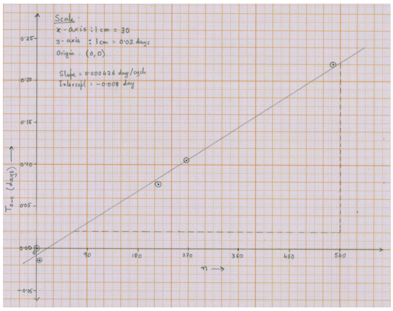
Hand-drawn graph D1.7 on graph paper: T_O−C (days) from −0.05 to 0.25 against n from 0 to 540, five circled points and a straight-line fit; notes: x-axis 1 cm = 30, y-axis 1 cm = 0.02 days, origin (0,0), slope = 0.000426 day/cycle, intercept = −0.008 day.

Plot uses more than 50% of graph paper: 0.5
Axes labels ( $T_{\mathrm{O-C}}$ and $n$ ) including dimensions: 0.5
Ticks and values on axes (or scale written explicitly): 0.5
Points correctly plotted: 0.5 for each point
Goodness of linear fit credited in next part

(D1.7d)

A linear fit to the plot of $T_{\mathrm{O-C}}$ vs $n$ gives the offset of period per cycle (slope) and the shift in the zero-phase point (intercept). [2.0]

This concept, which may be evident in the subsequent calculation, gains the credit, explicit statement is not necessary.

From a linear fit,

Slope $= 0.000\,43\ \mathrm{d/n} \qquad$ Intercept $= -0.010\ \mathrm{d}$ [3.0]

Credit for good visual linear fit: 1.0
Correct values of slope and intercept: 1.0 each
Tolerance: $\pm 0.00002$ in slope and $\pm 0.002$ in intercept.

T_{0,\mathrm{r}} = 5740.189 - 0.010 = \boxed{5740.179\ \mathrm{tMJD}}

[1.0]

P_{\mathrm{B,r}} = (1.12570 + 0.00043)\ \mathrm{d} = 1.126\,13\ \mathrm{d}

\boxed{P_{\mathrm{B}} = 1.1261\ \mathrm{d}}

[1.0]

Incorrect sign of correction applied carries penalty of 0.5 for each quantity.

Оригинал в Архива: Data-analysis-qp.pdf · официални решения: data_analysis_sol.pdf