Съдържание

Условие “Wobble” Method Transit Method Rocky or gaseous Transit light curves with starspots and limb darkening Решение

IOAA 2016, Теория, алтернативен вариант — Задача 12. T12. Exoplanets

Оригинал на условието (PDF)Съобщи за грешка

Всички материали от IOAA 2016

Exoplanets — alternate source edition · 50 т.

Внимание: Бележка към темата

This is the distinct T12 Exoplanets printed in both archived worked-key editions. Both separate question-paper editions instead print T12 AstroSat, preserved under ioaa-2016-theory-qp-p12. No chronology or final-version status is inferred. The Summary Answersheet and blank transit templates mentioned in T12.11–12 were not found in the inspected year inventory; the complete supplied answer diagrams and rubrics are retained.

Table of Constants

Fundamental Constants

Name	Symbol	Value
Speed of light in vacuum	$c$	$2.998\times10^8\ \mathrm{m\,s^{-1}}$
Planck constant	$h$	$6.626\times10^{-34}\ \mathrm{J\,s}$
Boltzmann constant	$k_B$	$1.381\times10^{-23}\ \mathrm{J\,K^{-1}}$
Stefan-Boltzmann constant	$\sigma$	$5.670\times10^{-8}\ \mathrm{W\,m^{-2}\,K^{-4}}$
Elementary charge	$e$	$1.602\times10^{-19}\ \mathrm{C}$
Gravitational constant	$G$	$6.674\times10^{-11}\ \mathrm{N\,m^2\,kg^{-2}}$
Gas constant	$R$	$8.315\ \mathrm{J\,mol^{-1}\,K^{-1}}$
Avogadro constant	$N_A$	$6.022\times10^{23}\ \mathrm{mol^{-1}}$
Wien's displacement constant	$\lambda_mT$	$2.898\times10^{-3}\ \mathrm{m\,K}$
Mass of electron	$m_e$	$9.109\times10^{-31}\ \mathrm{kg}$
Mass of proton	$m_p$	$1.673\times10^{-27}\ \mathrm{kg}$
Mass of neutron	$m_n$	$1.675\times10^{-27}\ \mathrm{kg}$
Atomic mass unit	$u$	$1.661\times10^{-27}\ \mathrm{kg}$

Astronomical Constants

Name	Symbol	Value
Parsec	pc	$3.086\times10^{16}\ \mathrm{m}$
Astronomical unit	$a_\oplus$	$1.496\times10^{11}\ \mathrm{m}$
Mass of the Sun	$M_\odot$	$1.989\times10^{30}\ \mathrm{kg}$
Radius of the Sun	$R_\odot$	$6.955\times10^8\ \mathrm{m}$
Luminosity of the Sun	$L_\odot$	$3.826\times10^{26}\ \mathrm{W}$
Apparent magnitude of the Sun at midday		$-26.72\ \mathrm{mag}$
Solar constant		$1366\ \mathrm{W\,m^{-2}}$
Angular diameter of the Sun		$30'$
Mass of the Earth	$M_\oplus$	$5.972\times10^{24}\ \mathrm{kg}$
Radius of the Earth	$R_\oplus$	$6.371\times10^6\ \mathrm{m}$
Tropical year		$365.242$ solar days $=3.156\times10^7\ \mathrm{s}$

Условие

Two major methods of detection of exoplanets (planets around stars other than the Sun) are the radial velocity (or so-called “wobble”) method and the transit method. In this problem, we find out how a combination of the results of these two methods can reveal a lot of information about an orbiting exoplanet and its host star.

Throughout this problem, we consider the case of a planet of mass $M_p$ and radius $R_p$ moving in a circular orbit of radius $a$ around a star of mass $M_s$ ( $M_s\gg M_p$ ) and radius $R_s$ . The normal to the orbital plane of the planet is inclined at angle $i$ with respect to the line of sight ( $i=90^\circ$ would mean “edge on” orbit). We assume that there is no other planet orbiting the star and $R_s\ll a$ .

“Wobble” Method

When a planet and a star orbit each other around their barycentre, the star is seen to move slightly, or “wobble”, since the centre of mass of the star is not coincident with the barycentre of the star-planet system. As a result, the light received from the star undergoes a small Doppler shift related to the velocity of this wobble.

The line of sight velocity, $v_l$ , of the star can be determined from the Doppler shift of a known spectral line, and its periodic variation with time, $t$ , is shown in the schematic diagram below. In the diagram, the two measurable quantities in this method, namely, the orbital period $P$ and maximum line of sight velocity $v_0$ are shown.

Periodic stellar line-of-sight velocity, with amplitude v_0 and period P.

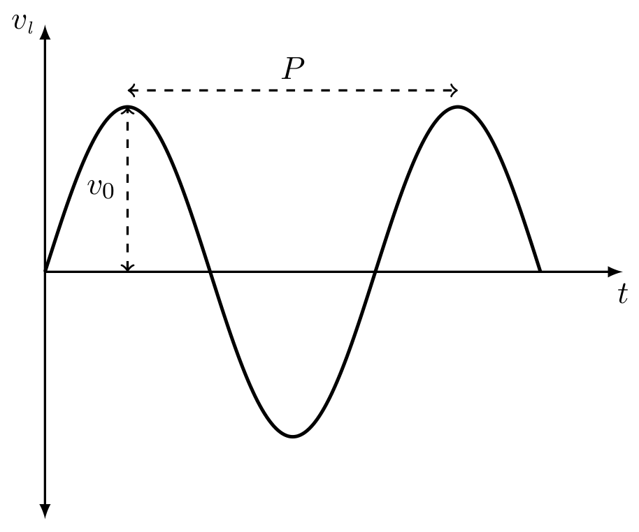
T12.1 Derive expressions for the orbital radius ( $a$ ) and orbital speed ( $v_p$ ) of the planet in terms of $M_s$ and $P$ . [3 т.]

T12.2 Obtain a lower limit on the mass of the planet, $M_{p,\min}$ in terms of $M_s$ , $v_0$ and $v_p$ . [4 т.]

Transit Method

As a planet orbits its host star, for orientations of the orbital plane that are close to “edge-on” ( $i\approx90^\circ$ ), it will pass periodically, or “transit”, in front of the stellar disc as seen by the observer. This would cause a tiny decrease in the observed stellar flux which can be measured. The schematic diagram below (NOT drawn to scale) shows the situation from the observer’s perspective and the resulting transit light curve (normalised flux, $f$ , vs time, $t$ ) for a uniformly bright stellar disc.

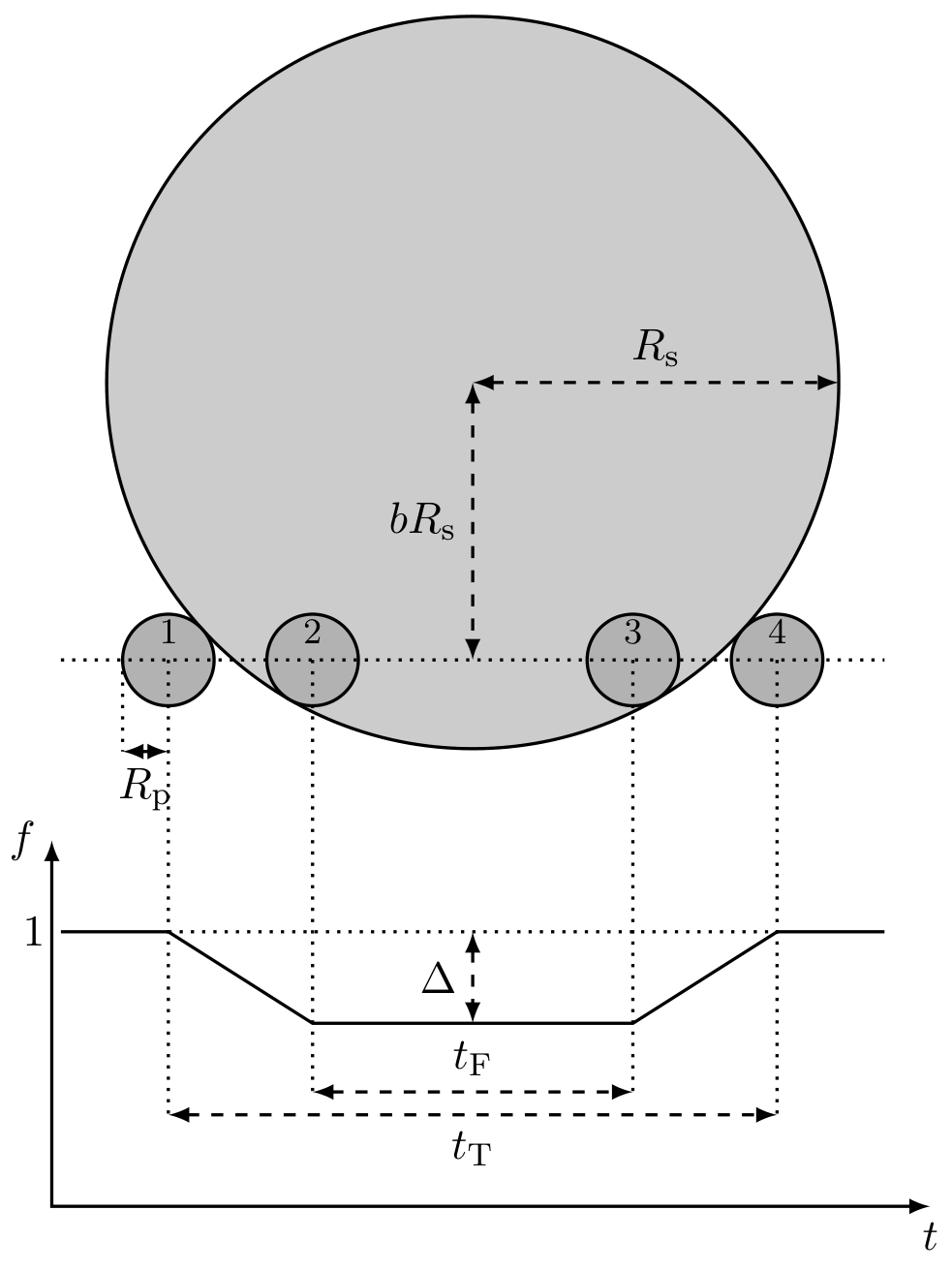
Transit contacts, stellar and planetary radii, impact parameter and light curve with transit durations and depth.

If the inclination angle $i$ is exactly $90^\circ$ , the planet would be seen to cross the stellar disc along a diameter. For other values of $i$ , the transit occurs along a chord, whose centre lies at a distance $bR_s$ from the centre of the stellar disc, as shown. The no-transit flux is normalised to 1 and the maximum dip during the transit is given by $\Delta$ .

The four significant points in the transit are the first, second, third and fourth contacts, marked by the positions 1 to 4, respectively, in the figure above. The time interval during the second and third contacts is denoted by $t_F$ , when the disc of the planet overlaps the stellar disc fully. The time interval between the first and fourth contacts is denoted by $t_T$ .

These points are also marked in the schematic diagram below showing a “side-on” view of the orbit (NOT drawn to scale).

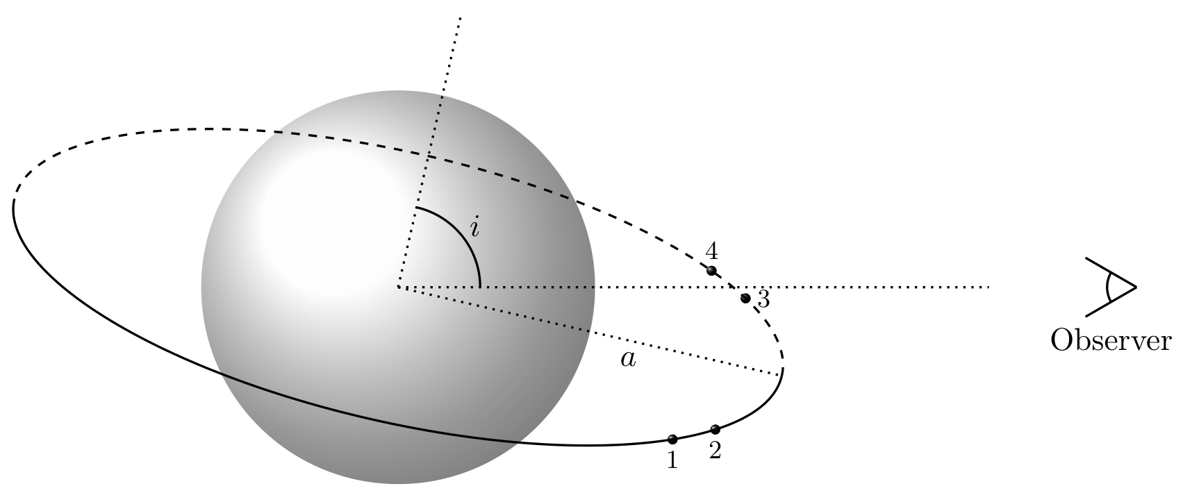
Side-on orbit with inclination, radius, contact positions and observer.

The measurable quantities in the transit method are $P$ , $t_T$ , $t_F$ and $\Delta$ .

T12.3 Find the constraint on $i$ in terms of $R_s$ and $a$ for the transit to be visible at all to the distant observer. [2 т.]

T12.4 Express $\Delta$ in terms of $R_s$ and $R_p$ . [1 т.]

T12.5 Express $t_T$ and $t_F$ in terms of $R_s$ , $R_p$ , $a$ , $P$ and $b$ . [8 т.]

T12.6 In the approximation of an orbit much larger than the stellar radius, show that the parameter $b$ is given by

b=\left[1+\Delta-2\sqrt{\Delta}\frac{1+(t_F/t_T)^2}{1-(t_F/t_T)^2}\right]^{1/2}

[5 т.]

T12.7 Use the result of part (T12.6) to obtain an expression for the ratio $a/R_s$ in terms of measurable transit parameters, using a suitable approximation. [3 т.]

T12.8 Combine the results of the wobble method and the transit method to determine the stellar mean density $\rho_s\equiv\frac{M_s}{4\pi R_s^3/3}$ in terms of $t_T$ , $t_F$ , $\Delta$ and $P$ . [6 т.]

Rocky or gaseous

Let us consider an edge-on ( $i=90^\circ$ ) star-planet system (circular orbit for the planet), as seen from the Earth. It is known that the host star is of mass $1.00M_\odot$ . Transits are observed with a period ( $P$ ) of 50.0 days and total transit duration ( $t_T$ ) of 1.00 hour. The transit depth ( $\Delta$ ) is 0.0064. The same system is also observed in the wobble method to have a maximum line of sight velocity of $0.400\ \mathrm{m\,s^{-1}}$ .

T12.9 Find the orbital radius $a$ of the planet in units of AU and in metres. [2 т.]

T12.10 Find the ratio $t_F/t_T$ of the system. [2 т.]

T12.11 Obtain the mass $M_p$ and radius $R_p$ of the planet in terms of the mass ( $M_\oplus$ ) and radius ( $R_\oplus$ ) of the Earth respectively. Is the composition of the planet likely to be rocky or gaseous? Tick the box for ROCKY or GASEOUS in the Summary Answersheet. [8 т.]

Transit light curves with starspots and limb darkening

T12.12 Consider a planetary transit with $i=90^\circ$ around a star which has a starspot on its equator, comparable to the size of the planet, $R_p$ . The rotation period of the star is $2P$ . Draw schematic diagrams of the transit light curve for five successive transits of the planet (in the templates provided in the Summary Answersheet). The no-transit flux for each transit may be normalised to unity independently. Assume that the planet does not encounter the starspot on the first transit but does in the second. [4 т.]

T12.13 Throughout the problem we have considered a uniformly bright stellar disc. However, real stellar discs have limb darkening. Draw a schematic transit light curve when limb darkening is present in the host star. [2 т.]

Решение

T12.1

Kepler’s law:

a=\boxed{\left(\frac{GM_s}{4\pi^2}P^2\right)^{1/3}}

[1.0]

Gravitational force provides centripetal acceleration:

v_p=\sqrt{\frac{GM_s}{a}}

[0.5]

v_p=\boxed{\left(\frac{2\pi GM_s}{P}\right)^{1/3}}

[1.5]

T12.2

Momentum conservation:

M_pv_p=M_sv_s

[1.5]

Observed quantity is $v_0=v_s\sin i$ . Thus,

M_{p,\min}=M_p\sin i=\frac{M_sv_s\sin i}{v_p}=\boxed{\frac{M_sv_0}{v_p}}

This is a lower limit on $M_p$ . [2.5]

T12.3

bR_s=a\cos i

[1.0]

Therefore, for visibility, $0\le b\le1\Rightarrow i\ge\cos^{-1}(R_s/a)$ . [1.0]

T12.4

Blackbody $\Rightarrow$ brightness is proportional to area. Since the observer is far away from the star-planet system, size of silhouette of planet on stellar disc is independent of $a$ .

\Delta=\left(\frac{R_p}{R_s}\right)^2

[1.0]

T12.5

Circular orbit $\Rightarrow$ uniform orbital speed

\Rightarrow\frac{t}{P}=\frac{a\phi}{2\pi a}=\frac{\phi}{2\pi}

[1.0]

where $\phi$ is the angle subtended by the planet at the centre of the star during transit (over time $t$ ).

Transit chord geometry and orbital angles for contact pairs 1–4 and 2–3.

(l_{23}/2)^2=(R_s-R_p)^2-(bR_s)^2

l_{23}=2R_s\sqrt{(1-R_p/R_s)^2-b^2}

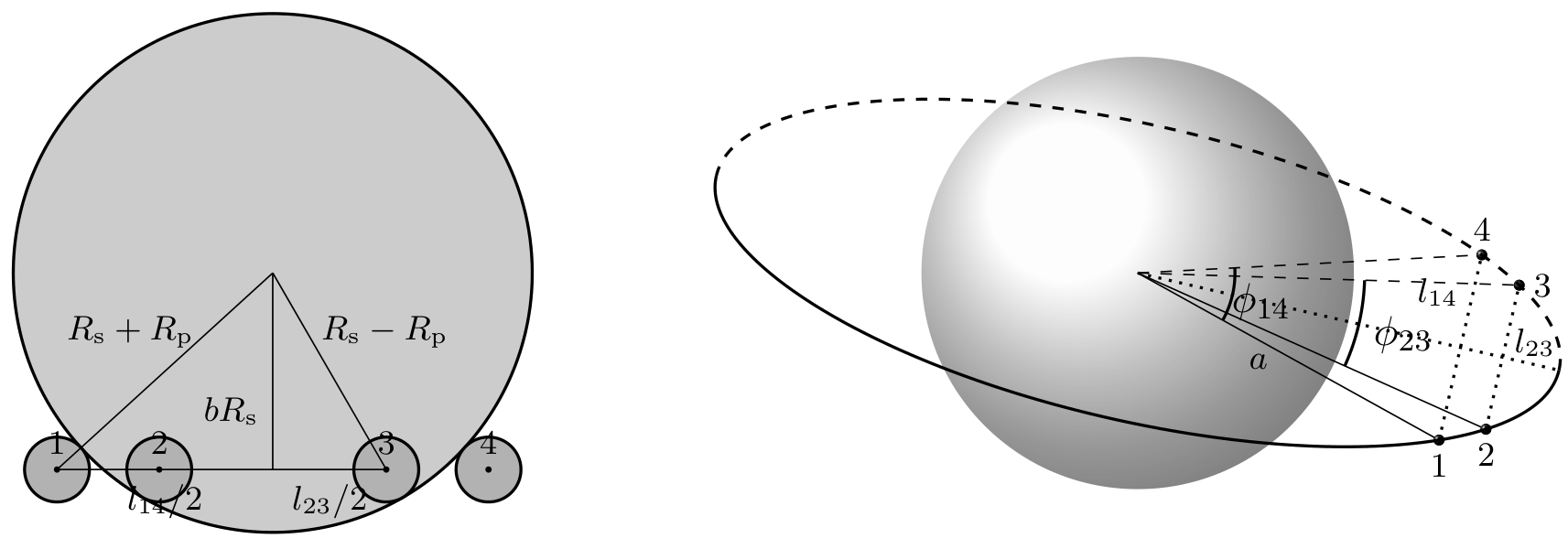
[2.0]

\sin(\phi_{23}/2)=\frac{l_{23}/2}{a}

[2.0]

\Rightarrow\phi_{23}=2\sin^{-1}\left(\frac{l_{23}}{2a}\right)=2\sin^{-1}\left[\frac{R_s}{a}\sqrt{\left(1-\frac{R_p}{R_s}\right)^2-b^2}\right]

[1.0]

t_F=\frac{P}{2\pi}\phi_{23}=\frac{P}{\pi}\sin^{-1}\left[\frac{R_s}{a}\sqrt{\left(1-\frac{R_p}{R_s}\right)^2-b^2}\right]

[1.0]

Similarly,

t_T=\frac{P}{\pi}\sin^{-1}\left[\frac{R_s}{a}\sqrt{\left(1+\frac{R_p}{R_s}\right)^2-b^2}\right]

[1.0]

T12.6

Since $R_s\ll a$ , use $\sin^{-1}x\approx x$ . [2.0]

t_T\approx\frac{P}{\pi}\left[\frac{R_s}{a}\sqrt{\left(1+\frac{R_p}{R_s}\right)^2-b^2}\right]

t_F\approx\frac{P}{\pi}\left[\frac{R_s}{a}\sqrt{\left(1-\frac{R_p}{R_s}\right)^2-b^2}\right]

Dividing, and putting $R_p/R_s=\sqrt{\Delta}$ ,

\frac{t_F}{t_T}=\left[\frac{(1-\sqrt{\Delta})^2-b^2}{(1+\sqrt{\Delta})^2-b^2}\right]^{1/2}

[1.0]

\Rightarrow b=\left[\frac{(1-\sqrt{\Delta})^2-(t_F/t_T)^2(1+\sqrt{\Delta})^2}{1-(t_F/t_T)^2}\right]^{1/2}=\left[1+\Delta-2\sqrt{\Delta}\frac{1+(t_F/t_T)^2}{1-(t_F/t_T)^2}\right]^{1/2}

[2.0]

Expressions lacking the use of approximation $R_s/a\ll1$ , but otherwise correct will get a penalty of 2.0.

Use of approximation with proper justification at a later stage than at the first step will get full credit.

T12.7

t_T=\frac{P}{\pi}\left[\frac{R_s}{a}\sqrt{\left(1+\frac{R_p}{R_s}\right)^2-b^2}\right]

[1.0]

Either substitution of $b$ or elimination of $b$ gets 1.0.

Substituting $b$ and $R_p/R_s$ ,

t_T=\frac{P}{\pi}\left[\frac{R_s}{a}\sqrt{(1+\sqrt{\Delta})^2-1-\Delta+2\sqrt{\Delta}\frac{1+(t_F/t_T)^2}{1-(t_F/t_T)^2}}\right]

\Rightarrow t_T=\frac{P}{\pi}\frac{R_s}{a}\left[\frac{4\sqrt{\Delta}}{1-(t_F/t_T)^2}\right]^{1/2}

\Rightarrow\frac{a}{R_s}=\frac{2P\Delta^{1/4}}{\pi(t_T^2-t_F^2)^{1/2}}

[2.0]

Expressions lacking the use of approximation $R_s/a\ll1$ , but otherwise correct will get a penalty of 1.0.

If penalty has already been imposed in part (T12.6), no further penalty for lack of approximation.

T12.8

From part (T12.7)

a=R_s\frac{2P\Delta^{1/4}}{\pi(t_T^2-t_F^2)^{1/2}}

From part (T12.1)

a=\left(\frac{GM_s}{4\pi^2}P^2\right)^{1/3}

Combining,

\frac{GM_s}{4\pi^2}P^2=\left[R_s\frac{2P\Delta^{1/4}}{\pi(t_T^2-t_F^2)^{1/2}}\right]^3

[3.0]

Identifying the two equations for combining gets credit. No credit for writing only one equation or irrelevant equations.

\Rightarrow\rho_s\equiv\frac{M_s}{4\pi R_s^3/3}=\frac{3}{4\pi}\frac{4\pi^2}{P^2G}\frac{8P^3\Delta^{3/4}}{\pi^3(t_T^2-t_F^2)^{3/2}}

[2.0]

\Rightarrow\boxed{\rho_s=\frac{24}{\pi^2G}\frac{P(\Delta)^{3/4}}{(t_T^2-t_F^2)^{3/2}}}

[1.0]

T12.9

From Kepler’s third law (with same mass of host star):

\frac{a}{a_\oplus}=\left(\frac{P}{P_\oplus}\right)^{2/3}

[1.0]

a=\left(\frac{50.0}{365.242}\right)^{2/3}\times1\ \mathrm{AU}=\boxed{0.266\ \mathrm{AU}}

[0.5]

=0.266\times1.496\times10^{11}\ \mathrm m=\boxed{3.97\times10^{10}\ \mathrm m}

[0.5]

T12.10

Edge-on $\Rightarrow b=0$ [1.0]

\frac{t_F}{t_T}=\left[\frac{(1-\sqrt{\Delta})^2-b^2}{(1+\sqrt{\Delta})^2-b^2}\right]^{1/2}=\frac{1-\sqrt{\Delta}}{1+\sqrt{\Delta}}=\boxed{0.8519}

[1.0]

T12.11

From parts (T12.1) and (T12.9)

v_{\mathrm{p}} = \sqrt{\frac{GM_{\odot}}{a}} = \sqrt{\frac{6.674 \times 10^{-11} \times 1.989 \times 10^{30}}{3.97 \times 10^{10}}} = 57.798\ \mathrm{km\ s^{-1}}

[1.0]

Assumption of small planet ( $M_{\mathrm{p}} \ll M_{\mathrm{s}}$ ) is valid because $\Delta$ is very small; less dense planet would make the assumption stronger!

M_{\mathrm{p}} = \frac{M_{\mathrm{s}}v_0}{v_{\mathrm{p}}} = \frac{1.989 \times 10^{30} \times 0.400}{5.7798 \times 10^{4} \times 5.972 \times 10^{24}} M_{\oplus} = \boxed{2.30\ M_{\oplus}}

[2.0]

From part (T12.4),

R_{\mathrm{p}} = R_{\mathrm{s}}\sqrt{\Delta}

From part (T12.7),

\frac{a}{R_{\mathrm{s}}} = \frac{2P\Delta^{1/4}}{\pi(t_{\mathrm{T}}^{2} - t_{\mathrm{F}}^{2})^{1/2}} = \frac{2P\Delta^{1/4}}{\pi t_{\mathrm{T}}(1 - (t_{\mathrm{F}}/t_{\mathrm{T}})^{2})^{1/2}}

\therefore\ R_{\mathrm{s}} = \frac{a\pi t_{\mathrm{T}}(1 - (t_{\mathrm{F}}/t_{\mathrm{T}})^{2})^{1/2}}{2P\Delta^{1/4}}

Combining,

R_{\mathrm{p}} = \frac{a\pi t_{\mathrm{T}}(1 - (t_{\mathrm{F}}/t_{\mathrm{T}})^{2})^{1/2}\Delta^{1/2}}{2P\Delta^{1/4}}

= \frac{a\pi t_{\mathrm{T}}(1 - (t_{\mathrm{F}}/t_{\mathrm{T}})^{2})^{1/2}\Delta^{1/4}}{2P}

[2.0]

= \frac{3.97 \times 10^{10} \times \pi \times \frac{1}{24} \times (1 - 0.8519^{2})^{1/2} \times (0.0064)^{1/4}}{2 \times 50.0 \times 6.371 \times 10^{6}} R_{\oplus}

= \boxed{1.21\ R_{\oplus}}

[1.0]

Mean density

\rho_{\mathrm{p}} = \frac{M_{\mathrm{p}}}{4\pi R_{\mathrm{p}}^{3}/3} = \frac{2.30}{(1.21)^{3}} \rho_{\oplus} = 1.3\rho_{\oplus}

[1.0]

Since mean density is higher than that of Earth, the planet is $\boxed{\mathrm{Rocky}}$ . [1.0]

T12.12

Five successive transit light curves, with a starspot spike in the second and fourth transit only.

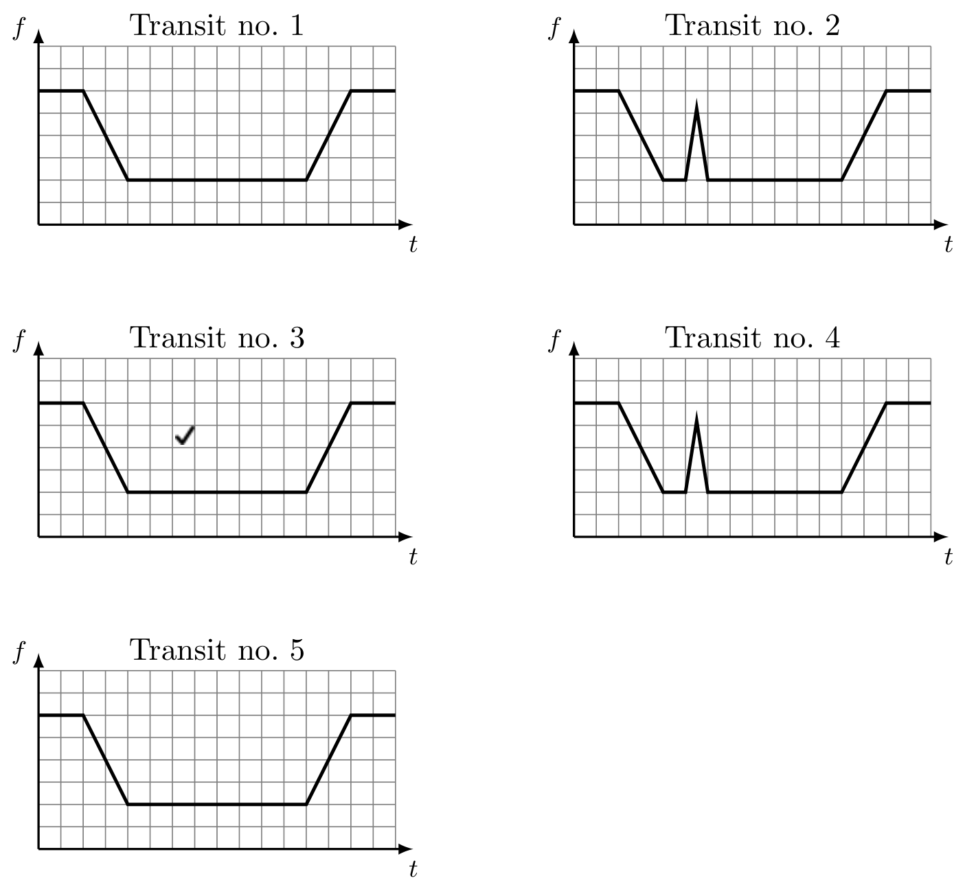
No change in the first: 0.5
Spike in second (width and phase of spike is arbitrary): 1.0
Height of spike (almost) equal to maximum dip: 0.5
No change in third: 0.5
Spike again in fourth: 0.5
Same phase of spike in second and fourth: 0.5
No change in 5th: 0.5

T12.13

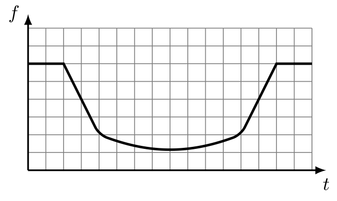
Transit light curve with limb darkening: rounded bottom and central minimum.

Non-flat bottom with central minimum gets 2.0. Curvature of ingress and egress are tolerated.

Оригинал в Архива: theory_sol.pdf · официални решения: theory_sol.pdf · допълнителни данни: theory.pdf · допълнителни данни: tableofconstants.pdf