IOAA 2017, Анализ на данни — Задача 1. Calibrating the distance ladder to the LMC
Data Analysis Examination · 75 т.
Указания
- The data analysis examination lasts for 4 hours and is worth a total of 150 marks.
- Dedicated IOAA Summary Answer Sheets are provided for writing your answers. Enter the final answers into the appropriate boxes in the corresponding Summary Answer Sheet. On each Answer Sheet, please fill in
- Student Code (Country Code and 1 digit)
- Graph Papers are required for your solutions. On each Graph Paper, please fill in
- Student Code (Country Code and 1 digit)
- Question no.
- Graph no. and total number of graph papers used.
- There are Answer Sheets for carrying out detailed work/rough work. On each Answer Sheet, please fill in
- Student Code (Country Code and 1 digit)
- Question no.
- Page no. and total number of pages.
- Start each problem on a separate Answer Sheet. Please write only on the printed side of the sheet. Do not use the reverse side. If you have written something on any sheet which you do not want to be evaluated, cross it out.
- Use as many mathematical expressions as you think that may help the evaluator to better understand your solutions. The evaluator may not understand your language. If it is necessary to explain something in words, please use short phrases (if possible in English).
- You are not allowed to leave your working desk without permission. If you need any assistance (malfunctioning calculator, need to visit a restroom, need more Answer Sheets, etc.), please draw the attention of the invigilator using the sign card.
- The beginning and end of the examination will be indicated by a long sound signal. Additionally, there will be a buzzer sound, fifteen minutes before the end of the examination (before the final sound signal).
- At the end of the examination you must stop writing immediately. Sort and put your Summary Answer Sheets, Graph Papers, and Answer Sheets for each part (D1 and D2) in separate stack. You are not allowed to take any sheet of paper out of the examination area.
- Wait at your table until your envelope is collected. Once all envelopes are collected, your student guide will escort you out of the examination area.
- A list of constants is given on the next page.
Table of constants
| Mass () | kg | Earth |
| Radius () | m | |
| Acceleration of gravity () | 9.8 m s | |
| Obliquity of Ecliptic | 23°27’ | |
| Length of Tropical Year | 365.2422 mean solar days | |
| Length of Sidereal Year | 365.2564 mean solar days | |
| Albedo | 0.39 | |
| Mass(M☾) | kg | Moon |
| Radius (R☾) | m | |
| Mean distance from Earth | m | |
| Orbital inclination with the Ecliptic | 5.14° | |
| Albedo | 0.14 | |
| Apparent magnitude (mean full moon) | -12.74 | |
| Mass () | kg | Sun |
| Radius () | m | |
| Luminosity () | W | |
| Absolute Magnitude () | 4.80 mag | |
| Angular diameter | 0.5 degrees | |
| 1 au | m | Physical constants |
| 1 pc | 206,265 au | |
| Distance from Sun to Barnard’s Star | 1.83 pc | |
| Gravitational constant () | ||
| Planck constant () | ||
| Boltzmann constant () | ||
| Stefan-Boltzmann constant () | ||
| Hubble constant () | 72 km s Mpc | |
| Speed of light in vacuum () | 299,792,458 m s | |
| Proton mass | 938.27 MeV c | |
| Deuterium mass | 1875.60 MeV c | |
| Neutron mass | 939.56 MeV c | |
| Helium-3 mass | 2808.30 MeV c | |
| Helium-4 mass | 3727.40 MeV c |
Условие
An accurate trigonometric parallax calibration for Galactic Cepheids has long been sought, but is very difficult to achieve in practice. All known classical (Galactic) Cepheids are more than 250 pc away, therefore for direct distance estimates to achieve an uncertainty of up to 10%, parallax uncertainties of up to ±0.2 milliarcsec are needed, requiring space-based observations. The Hipparcos satellite reported parallaxes for 200 of the nearest Cepheids, but even the best of these had high uncertainties. Recent progress has come with the use of the Fine Guidance Sensor on HST where parallaxes (in many cases) accurate to better than ±10% were obtained for 10 Cepheids, spanning a range of periods from 3.7 to 35.6 days. These nearby Cepheids cover distances from about 300 to 560 pc.
The measured periods, P, and average magnitudes in V, K and I bands are given in Table 1 as well as the and for extinction in V and K bands, respectively. The measured parallaxes with their uncertainties are also given in milliarcsec (mas). All measured apparent magnitudes have negligible uncertainty.
Table 1: Periods and average apparent magnitudes of 5 Galactic Cepheids with accurate parallax measurements.
| P (day) | (mag) | (mag) | (mag) | (mag) | (mag) | parallax (mas) | error (mas) | |
|---|---|---|---|---|---|---|---|---|
| RT Aur | 3.728 | 5.464 | 3.925 | 0.20 | 0.02 | 4.778 | 2.40 | 0.19 |
| FF Aql | 4.471 | 5.372 | 3.465 | 0.64 | 0.08 | 4.510 | 2.81 | 0.18 |
| X Sgr | 7.013 | 4.556 | 2.557 | 0.58 | 0.07 | 3.661 | 3.00 | 0.18 |
| ζ Gem | 10.151 | 3.911 | 2.097 | 0.06 | 0.01 | 3.085 | 2.78 | 0.18 |
| l Car | 35.551 | 3.732 | 1.071 | 0.52 | 0.06 | 2.557 | 2.01 | 0.20 |
(D1.1) The observed correlation between the period of a Cepheid and its brightness is usually described by the so-called “Period-Luminosity (PL) relation”, where . In fact, such a relation is normally expressed in terms of the period and absolute magnitude, instead of luminosity. Hereafter, we shall refer to the Period-Absolute magnitude relation as the conventionally named “PL relation”.
Use the data given in Table 1 to plot a suitable linear graph in order to derive the Cepheid PL relation for the V-band and K-band. You should plot each graph separately on different pieces of graph paper. Determine the slope of the line that best describes the linear relation of the data. (You may find the relation useful) [36,5 т.]
Any apparent differences in PL relations of stars in the different bands can be explained if one also considers differences in colour. Therefore, the PL relation is in fact a PLC (Period-Luminosity-Colour) relation. This is from the reddening effect, due to extinction being a function of wavelength, which can also vary among different Cepheids due to their different metallicities, foreground Interstellar Medium and dust.
A new reddening-free magnitude (or bandpass) called “Wesenheit” has been proposed that does not require the explicit information of the extinction of individual stars but uses colour information from the star itself to get rid of the effect. For example, use V and I band photometry and is defined as
where depends on the reddening law. In this case, we shall take the value of to be 2.45.
(D1.2) From the data given in Table 1, plot and derive the reddening-free PL relation using Wesenheit magnitudes. Estimate the linear slope of the relation as well as its uncertainty. [14,5 т.]
(D1.3) Next, we would like to use the newly-derived PL relations from question (D1.1) & (D1.2) to estimate the distance to the Large Magellenic Cloud (LMC) using periods and magnitudes of classical Cepheids in the LMC. In Table 2, the periods, average extinction-corrected apparent magnitudes, , and Wesenheit magnitudes are given.
Estimate the distance modulus, , to each star and then use all the information to derive the distance to the LMC (in parsecs) and its standard deviation for each band.
Compare if the derived distances are statistically different for the 2 bands (YES/NO).
Are the standard deviations of the estimated distances for 2 bands different (YES/NO)?
Based on this dataset, which band (V or Wesenheit) is more accurate in estimating the distance to the LMC? [24 т.]
Table 2: Period, average extinction-corrected apparent magnitude, , and average Wesenheit magnitude measurements of Cepheids in the LMC
| P (day) | mag | mag | |
|---|---|---|---|
| HV12199 | 2.63 | 16.08 | 14.56 |
| HV12203 | 2.95 | 15.93 | 14.40 |
| HV12816 | 9.10 | 14.30 | 12.80 |
| HV899 | 30.90 | 13.07 | 10.97 |
| HV2257 | 39.36 | 12.86 | 10.54 |
Отговори
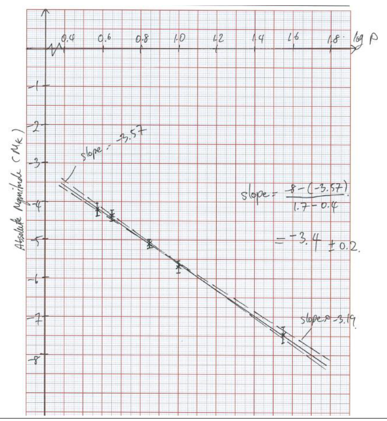
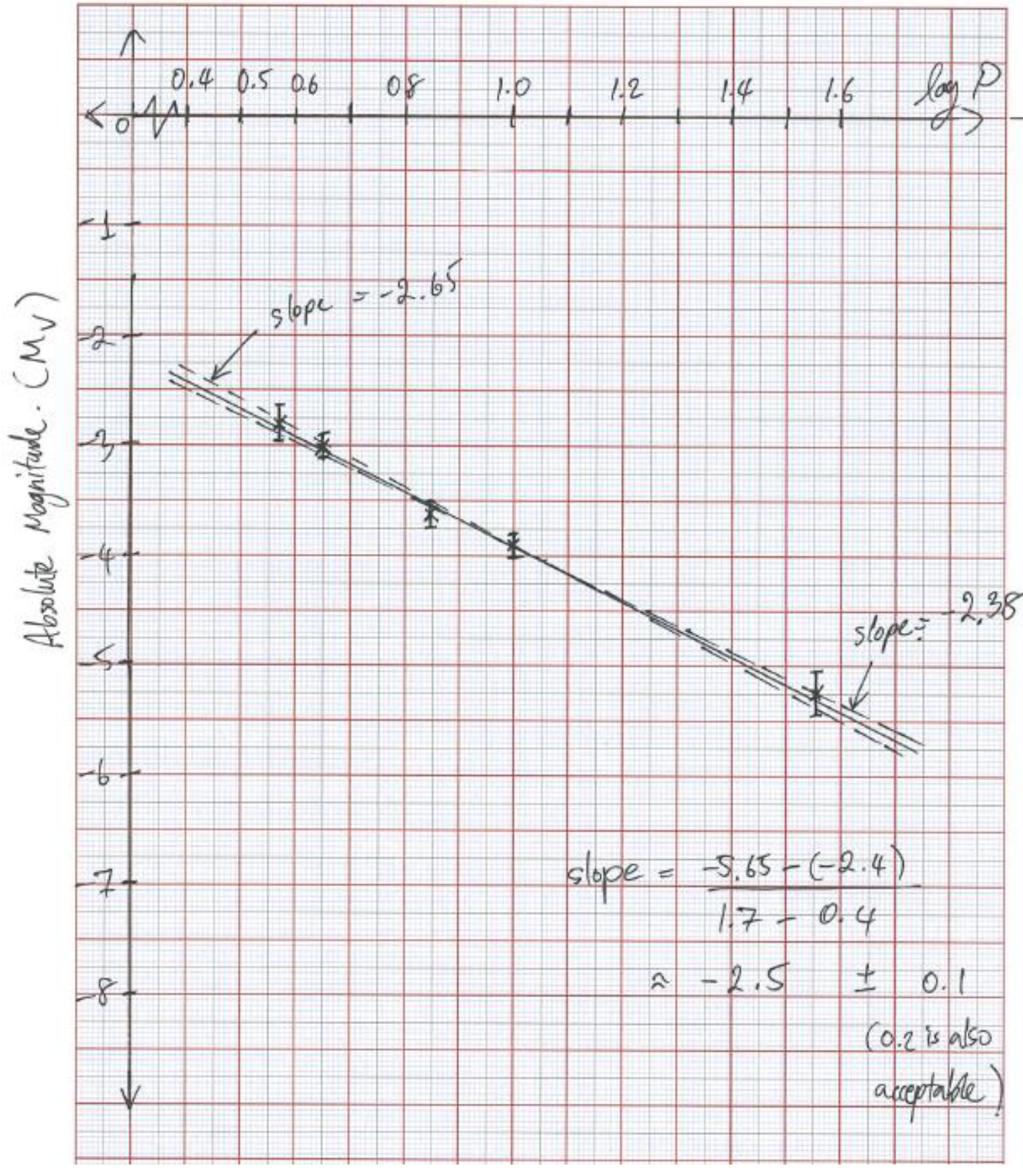
(D1.1) V-band slope ≈ −2.5 ± 0.1; K-band slope ≈ −3.4 ± 0.2
From the official solution graphs; the marking scheme accepts −2.5 ± 0.2 (V) and −3.4 ± 0.2 (K), with uncertainty between 0.1 and 0.3.
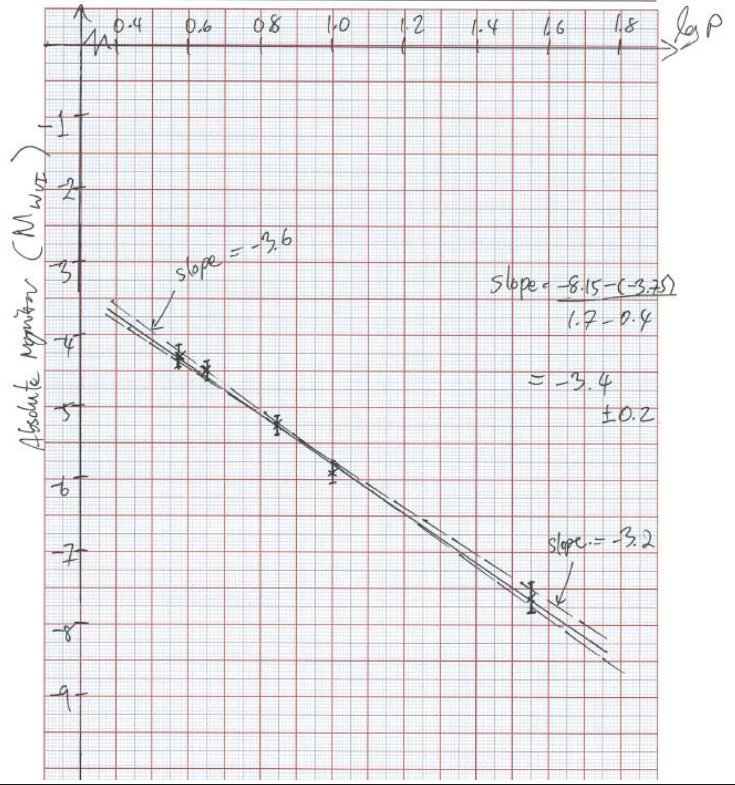
(D1.2) slope ≈ −3.4 ± 0.2
From the official solution graph for the bandpass.
(D1.3) V: 46170 ± 4116 pc; Wesenheit: 48068 ± 865 pc; distances not statistically different (NO); standard deviations different (YES); the Wesenheit magnitude is more accurate.
Values from the official solution table (mean and STD. of the per-star distances).
Решение
(D1) Calibrating distance ladder to the LMC [75 marks]
An accurate trigonometric parallax calibration for Galactic Cepheids has been long sought, but very difficult to achieve in practice. All known classical (Galactic) Cepheids are more than 250 pc away, therefore for direct distance estimates to have an uncertainty of up to 10%, parallax accuracies with uncertainties of up to ±0.2 milliarcsec are needed, requiring space observations. The Hipparcos satellite reported parallaxes for 200 of the nearest Cepheids, but even the best of these had high uncertainties. Recent progress has come with the use of the Fine Guidance Sensor on HST with parallaxes (in many cases) accurate to better than ±10% were obtained for 10 Cepheids, spanning the period range from 3.7 to 35.6 days. These nearby Cepheids span a range of distances from about 300 to 560 pc.
The measured periods, P, average magnitudes in V, K and I bands are given in Table 1 as well as the and for extinction in V and K bands, respectively. The measured parallax with its uncertainty are also given in milliarcsec (mas). All measured apparent magnitude has negligibly small uncertainty.
Table 1: Period and average apparent magnitude of 5 Galactic Cepheids with accurate parallax measurements
| P (day) | (mag) | (mag) | (mag) | (mag) | (mag) | parallax (mas) | error (mas) | |
|---|---|---|---|---|---|---|---|---|
| RT Aur | 3.728 | 5.464 | 3.925 | 0.20 | 0.02 | 4.778 | 2.40 | 0.19 |
| FF Aql | 4.471 | 5.372 | 3.465 | 0.64 | 0.08 | 4.510 | 2.81 | 0.18 |
| X Sgr | 7.013 | 4.556 | 2.557 | 0.58 | 0.07 | 3.661 | 3.00 | 0.18 |
| ζ Gem | 10.151 | 3.911 | 2.097 | 0.06 | 0.01 | 3.085 | 2.78 | 0.18 |
| l Car | 35.551 | 3.732 | 1.071 | 0.52 | 0.06 | 2.557 | 2.01 | 0.20 |
(D1.1) The observed correlation between period of a Cepheid and its brightness is usually described by the so-called “Period-Luminosity (PL) relation” where . In fact, such relation is normally expressed in terms of period with the absolute magnitude instead of luminosity. Hereafter, we shall refer to Period-Absolute magnitude as the conventionally named “PL relation”.
Use the data given in Table 1 to plot a suitable linear graph in order to derive the Cepheid PL relation for V- and K-band. You should separately plot each graph on different piece of graph paper. Determine the slope of the linear line that best describe the linear relation of the data. (You may find the relation useful)
[39.5 Marks]
Solution:
For Cepheid variable the PL relation is
[1 Mark]
and recall that
so can be written in term of absolute magnitude,
and
subtract the 2 equations, we get
And from definition of absolute magnitude,
We therefore get the relation between vs. ,
Substitute in the PL relation, we get
or via realising that () [1 Mark]
where
-If student plot log L vs P, he/she should get slope which is (standard answer slope)/(-2.5). We already tell the student about using Absolute magnitude instead of Luminosity therefore half of the total marks should be deducted beyond this point if the student performs all corresponding calculations correctly.
- If the student plot absolute magnitude in reverse order and get positive slope but correct value for the slope, full mark should be awarded for the related parts
Calculate Absolute magnitude () and uncertainties from parallax and data in Table 1 for V & K
Calculate distances and uncertainties from
[2 mark]
And then calculate absolute magnitude and its uncertainty using
[2 mark]
- Calculate , , and and its error (30 x 0.5mark=15 Marks total, not including ) (if student does not explicitly write out values of , but get the correct answer for and its error, he/she should get full-mark for that parts)
- Calculate or from realizing that (0.5 Mark)
| logP | |||||||
|---|---|---|---|---|---|---|---|
| RT Aur | 416.6 | 32. | 0.572 | -2.83 | 0.17 | -4.19 | 0.17 |
| FF Aql | 355.8 | 22. | 0.650 | -3.02 | 0.13 | -4.37 | 0.13 |
| X Sgr | 333.3 | 20. | 0.846 | -3.63 | 0.13 | -5.12 | 0.13 |
| ζ Gem | 359.7 | 23. | 1.007 | -3.92 | 0.14 | -5.69 | 0.14 |
| l Car | 497.5 | 49. | 1.551 | -5.27 | 0.21 | -7.47 | 0.21 |
Plot Graph vs absolute magnitudes
- 2 plots x (5 point + 5 error bars) x 0.5 mark = 10 marks
- 2 plots x 2 axis (clearly labelled) x 0.5 mark= 2 marks
- 2 plots x Draw a straight line through data points and error bars x 1 mark = 2 marks
V-band,
Slope should be in the range
- 1 Mark if answer within -2.5+/-0.2 (half if within -2.5+/-0.3)
- uncertainty should be between 0.1-0.3 (1 mark)
K-band,
Slope should be in the range
- 1 Mark if answer within -3.4+/-0.2 (half if within -3.4+/-0.3)
- estimated uncertainty should be between 0.1-0.3 (1 mark)
Any apparent differences in PL relations of stars in different bands can be explained if one also considers differences in colour. Therefore, the PL relation is in fact a PLC (Period-Luminosity-Colour) relation. This is due to reddening effect that causes extinction as a function of wavelength which can also vary among different Cepheids due to their different metallicities, foreground Inter Stellar Medium and dust.
A new reddening-free magnitude (or bandpass) called “Wesenheit” has been proposed which does not require the explicit information of the extinction of individual star but uses colour information of the star itself to get rid of the effect. For example, use V and I band photometry and is defined as
where depends on the reddening law. In this case, we shall take the value of to be 2.45.
(D1.2) From the data given in Table 1, plot and derive reddening-free PL relation using Wesenheit magnitude. Estimate the linear slope of the relation as well as its uncertainty. [14.5 Marks]
Solution:
- Calculate the Wesenheit magnitude from the given V, I and values and then estimate the absolute magnitude for the Wesenheit system
| RT Aur | 3.78 | -4.31 |
| FF Aql | 3.26 | -4.49 |
| X Sgr | 2.36 | -5.25 |
| ζ Gem | 1.88 | -5.89 |
| l Car | 0.85 | -7.63 |
- calculate the values for and , 10 values x 0.5 = 5 marks (not including )
- Realising that or by full calculation 0.5 mark
- plot vs x (5 point + 5 error bars) )x 0.5 = 5 marks)
- 2 axis (labels, units) x 0.5 = 1 mark
- Draw appropriate straight line through the data or within error bar 1 mark
- 1 Mark for estimated slope within -3.4+/-0.2 (half if within -3.4+/-0.3)
- 1 Mark for estimated uncertainty of slope between 0.1-0.3
(D1.3) Next, we would like to use the newly derived PL relation from question (D1.1) & (D1.2) to estimate the distance to Large Magellenic Cloud (LMC) using periods and magnitudes of classical Cepheids in the LMC. In table 2, the periods, average extinction-corrected apparent magnitude, , and Wesenheit magnitudes are given.
Estimate distance modulus, , to each star and then use all the information to derive distance to LMC (in parsecs) and its standard deviation for each band. Compare if the derived distances are statistically different for the 2 bands (YES/NO). Are the standard deviations of the estimated distances for 2 bands different (YES/NO)? Based on this dataset, which band (V or Wesenheit) is more accurate in estimating the distance to LMC? [21 Marks]
Table 2: Period, average extinction-corrected apparent magnitude, , and average Wesenheit magnitude measurements of Cepheids in the LMC
| P (day) | mag | mag | |
|---|---|---|---|
| HV12199 | 2.63 | 16.08 | 14.56 |
| HV12203 | 2.95 | 15.93 | 14.40 |
| HV12816 | 9.10 | 14.30 | 12.80 |
| HV899 | 30.90 | 13.07 | 10.97 |
| HV2257 | 39.36 | 12.86 | 10.54 |
Solution:
Distance modulus in each band is given by
[0.5 Mark]
And from previous section
where we have estimated slope but not the intercept
Therefore, to get the distance in parsec we will need to evaluate
[1 Mark]
Using the best-estimate slope for each band and any point along the best-fit line (or intercept) student should be able to estimate
V-band: (1 mark if within +/-0.2, half if within +/-0.3)
band: (1 mark if within +/-0.2, half if within +/-0.3)
| Star | LogP | V distance (pc) | distance (pc) | ||
|---|---|---|---|---|---|
| HV12199 | 0.42 | 18.53 | 18.39 | 50813 | 47596 |
| HV12203 | 0.47 | 18.50 | 18.40 | 50223 | 47805 |
| HV12816 | 0.96 | 18.10 | 18.46 | 41640 | 49221 |
| HV899 | 1.49 | 18.19 | 18.43 | 43549 | 48660 |
| HV2257 | 1.60 | 18.25 | 18.36 | 44620 | 47058 |
| Mean | 46170 | 48068 | |||
| STD. | 4116 | 865 |
- calculate the values (, distance modulus, distance accurate to the nearest 100 pc) 25 x 0.5 mark=12.5 marks
- Calculate the mean (x 0.5 mark) and std. (x 0.5 mark) for each band (x2 bands) = 2 marks
a) Answer NO, the distances estimated from V and Wesenheit are not statistically different (1 mark)
- full mark: In case of “NO” and distances estimated from V- and -band are within 1 standard deviation of one another
- full mark: In case of “YES” and distances estimated from V- and -band are not within 1 standard deviation of one another but due to wrong numerical calculation from previous part (already penalised)
- Zero mark: in all cases if the answer is not consistent with reasoning similar to above
b) Answer YES, standard deviation in the estimated distances from the 2 bands are significantly different (1 mark)
- full mark: if the answer is consistent with the calculated std. when the answer is either “YES” or “NO”, “YES” if fractional uncertainty is similar and “NO” otherwise.
- zero mark: if the answer is not consistent with estimated uncertainties
c) Wessenheit magnitude is better at estimating the distance to LMC (1 marks)
- full mark: if answer is consistent with std.
- zero mark: otherwise
Оригинал в Архива: DataAnalysis.pdf · официални решения: DataAnalysis_Solution.pdf