Съдържание

IOAA 2019, Анализ на данни — Задача 1. Photometry and spectroscopy of Nova Del 2013

Оригинал на условието (PDF)Съобщи за грешка

Всички материали от IOAA 2019

Data analysis problem sheet · 60 т.

Условие

Classical nova V339 Del (Nova Delphini 2013) was discovered by Koichi Itagaki at 6.8 magnitude on 14 August 2013 at 14:01 UT (MJD = 56518.584). Both professional and amateur astronomers analysed the photometry and spectroscopy of the nova. Less than 10 hours after the alert, when the night falls at the Piszkéstető Mountain Station of the Konkoly Observatory of the Hungarian Academy of Sciences, Hungarian astronomers took the first spectrum data of the nova using the eShel echelle spectrograph in the Gothard Astrophysical Observatory of Loránd Eötvös University attached to the 1 meter telescope of the Konkoly Observatory.

Refer to Fig 1.1 and Fig 1.2 to complete the questions. The larger versions of Fig 1.1 and Fig 1.2 are found on separate A3 papers.

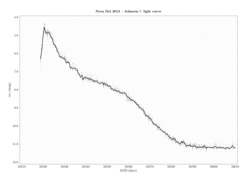
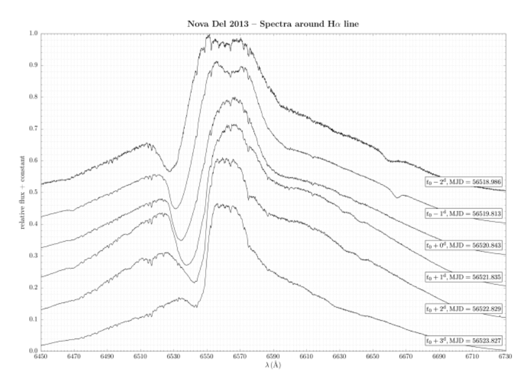
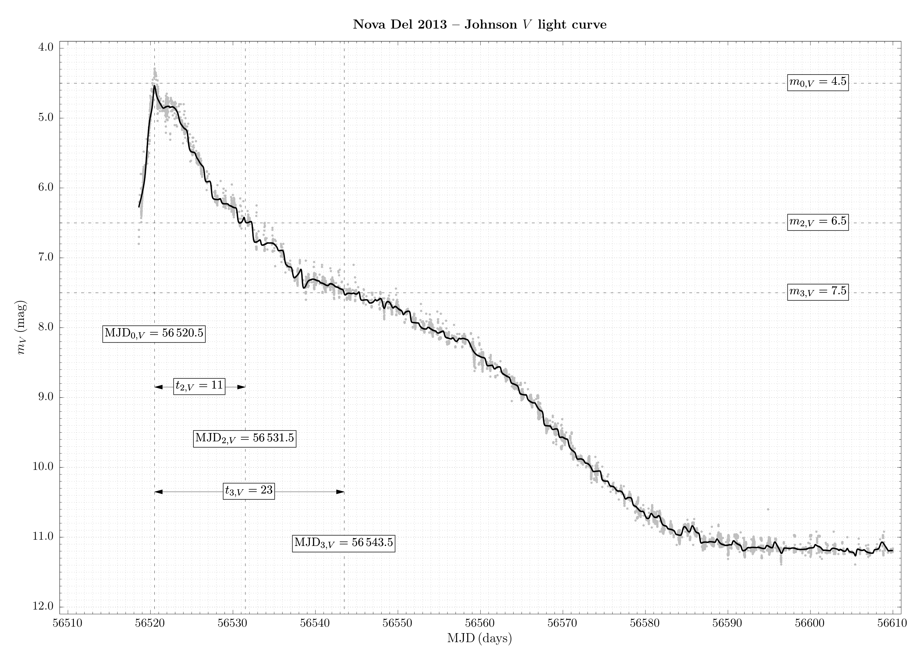
Light curve titled 'Nova Del 2013 – Johnson V light curve': V magnitude m_V (mag) from 4.0 (top) to 12.0 (bottom) against MJD (days) from 56510 to 56610; grey data points with a black smoothed line rising steeply to a peak near 4.5 mag just after MJD 56520, then declining to about 11.2 mag. — Fig. 1.1: Nova Del 2013 – Johnson V light curve

Fig. 1.2: Nova Del 2013 – Spectra around Hα line

Fig. 1.1 shows the visual light curve of the nova based on the data downloaded from the website of AAVSO (American Association of Variable Star Observers). On the horizontal and vertical axes, the Modified Julian Date (MJD = JD−2 400 000.5) of the observations and the Johnson V magnitudes are plotted, respectively. The grey circles (about 38000 data points) represent the measured values, while the continuous black line is the result of smoothing the data with a Gaussian filter (Full Width at Half Maximum = 0.5 day) to define an "average" light curve from the data points.

The rate of decline can be characterized by the values $t_2$ and $t_3$ , which show the time interval in days in which a nova fades from its maximum brightness by 2 and 3 magnitudes.

A few empirical formulae between the peak of the absolute magnitude in the $V$ band ( $M_0$ ) and $t_2$ , $t_3$ values can be found in the following literature:

(a) $M_0 = -7.92 - 0.81 \arctan \frac{1.32 - \log t_2}{0.23}$ (Della Valle, M. & Livio, M.: 1995, ApJ 452, 704)

(b) $M_0 = -11.32 + 2.55 \log t_2$ (Downes, R.A. & Durbeck, H.W.: 2000, AJ 120, 2007)

The $E(B-V)$ color excess of Nova Del 2013 (Chochol, D. et al.: 2014, Contrib. Astron. Obs. Skalnaté Pleso 43, 330) is:

E(B-V) = 0.184 \pm 0.035

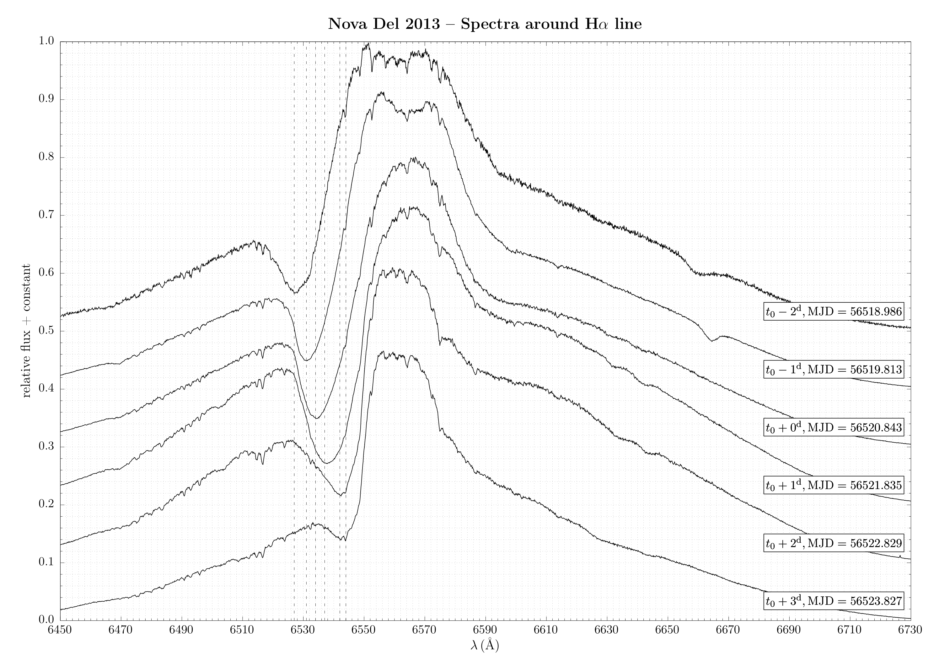
Fig 1.2 shows the nova spectra taken in the wavelength region around the H $\alpha$ line on six consecutive nights before and after the time of the maximum brightness ( $t_0$ ). The individual spectra have been shifted vertically for clarity. The Modified Julian Dates (MJD) of the observations are listed on the right hand side of each spectrum slice.

The H $\alpha$ line shows the so-called P Cygni profile with very broad wings, which is typical not of novae only, but is present in almost all spectral types and is a reliable sign of a massive radial motion of matter ejected from the star. The P Cygni profile is composed of a strong, broad emission peak which is considered to be centered at the rest wavelength in air $\lambda_0$ of the line – for H $\alpha$ $\lambda_0 = 6562.82\ \text{Å}$ – and a usually weaker, blueshifted absorption component. The expansion (radial) velocity of the shell can be approximated from the measured wavelength $\lambda$ of the absorption peak using the well known Doppler formula connecting the displacement $\Delta\lambda = \lambda - \lambda_0$ , the radial velocity $v_{\mathrm{r}}$ , and $c$ , the speed of light.

Assume that the H $\alpha$ line showing P Cygni profile is excited in the outermost part of the spherically expanding shell, and its extent at the moment of taking the first spectrum was still negligible.

a) From Fig. 1.1, estimate the Modified Julian Date of the peak magnitude ( $\mathrm{MJD}_0$ ) and the value of the peak magnitude itself. Consider the error of this brightness value to be $0.05^{\mathrm{m}}$ . [3 т.]

b) Estimate the Modified Julian Dates based on the time interval (days) in which the nova has faded by 2 and 3 magnitudes, then calculate $t_2$ and $t_3$ values. [6 т.]

c) With reference to $t_2$ and $t_3$ from (b), determine the peak absolute magnitude of the nova using all three empirical formulae listed earlier, calculate their mean ( $M_0$ ) and their standard deviation, and consider this latter as the uncertainty of $M_0$ .

The formula for standard deviation:

\sigma = \sqrt{\frac{\sum_{i=1}^{n} (x_i - \bar{x})^2}{n-1}}

[5 т.]

d) Using the value of the color excess $E(B-V)$ , determine the interstellar extinction $A_V$ and its uncertainty in the direction of the nova. Use $R_V = 3.1$ , without error. [4 т.]

e) Estimate the distance to the nova and its uncertainty. Give the result in kpc. [11 т.]

f) Measure the central wavelengths of the P Cygni absorption features plotted in Fig. 1.2 (refer to magnified version), and calculate the corresponding radial velocities. No error estimation is needed. [14 т.]

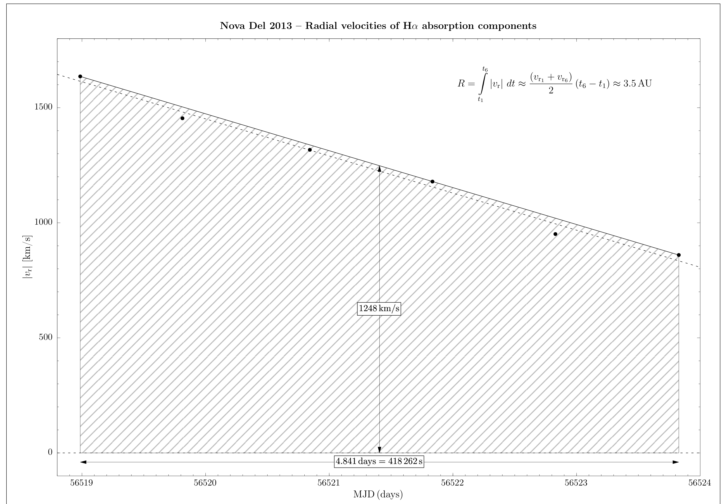
g) Plot these radial velocities against the Modified Julian Dates of the observations. [6 т.]

h) From the graph in (g), estimate the physical radius of the envelope at the end of the time interval. Give the answer in astronomical units (au). [7 т.]

i) Knowing the distance to the nova and the physical radius of the spherical envelope 5 days after the discovery, estimate the apparent angular diameter of the envelope then. [4 т.]

Отговори

Решение

a) From the light curve plot the Modified Julian Dates can be read with an error of about 0.5. The peak of the maximum brightness is very narrow and obviously placed at $\mathrm{MJD}_0 = 56\,520.5$ with a value of $m_0 = 4.5^{\mathrm{m}}$ , therefore:

$\mathrm{MJD}_0 = \boxed{56\,520.5 \pm 0.5}$ (2 p)

$m_0 = \boxed{4.5^{\mathrm{m}} \pm 0.05^{\mathrm{m}}}$ (1 p)

b) The brightness values of $2^{\mathrm{m}}$ and $3^{\mathrm{m}}$ decline are $6.5^{\mathrm{m}} \pm 0.05^{\mathrm{m}}$ and $7.5^{\mathrm{m}} \pm 0.05^{\mathrm{m}}$ , respectively. (2 p)

The corresponding Modified Julian Dates are $\mathrm{MJD}_2$ and $\mathrm{MJD}_3$ . Because of the poorly defined slopes on the light curve around these dates, their acceptable error is larger than in other parts of the light curve, let say it is about $1^{\mathrm{d}}$ , so:

$\mathrm{MJD}_2 = \boxed{56\,531.5 \pm 1}$ , $\quad \mathrm{MJD}_3 = \boxed{56\,543.5 \pm 1}$ (2 p)

$t_2 = \boxed{11^{\mathrm{d}} \pm 1^{\mathrm{d}}}$ , $\quad t_3 = \boxed{23^{\mathrm{d}} \pm 1^{\mathrm{d}}}$ (2 p)

c) The text of this part does not ask for calculating the individual errors of the formulae, but it is worth estimating them here, just for the sake of completeness. (Students won’t do it.)

(a) The form of the function is

M = a + b \arctan \frac{c - \log t_2}{d}, \quad a = -7.92, b = -0.81, c = 1.32, d = 0.23, \qquad (1.1)

so its derivative:

M' = -\frac{b}{d \log(10) \left[1 + \left(\frac{c - \log t_2}{d}\right)^2\right]} \frac{1}{t_2} \to \Delta M = -\frac{b}{d \log(10) \left[1 + \left(\frac{c - \log t_2}{d}\right)^2\right]} \frac{\Delta t_2}{t_2} \qquad (1.2)

The value and its error calculated from the formulae above (error is not necessary):

$M_0^{(a)} = \boxed{-8.63^{\mathrm{m}} \pm 0.06^{\mathrm{m}}}$ (1 p)

(b) The form of the function is

M = a + b \log t_2, \quad a = -11.32, b = 2.55 \qquad (1.3)

so its derivative:

M' = \frac{b}{t_2 \log(10)} \to \Delta M = \frac{b}{\log(10)} \frac{\Delta t_2}{t_2} \qquad (1.4)

The value and its error calculated from the formulae above (error is not necessary):

$M_0^{(b)} = \boxed{-8.66^{\mathrm{m}} \pm 0.10^{\mathrm{m}}}$ (1 p)

M = a + b \log t_3, \quad a = -11.99, b = 2.54 \qquad (1.5)

so its derivative:

M' = \frac{b}{t_3 \log(10)} \to \Delta M = \frac{b}{\log(10)} \frac{\Delta t_3}{t_3} \qquad (1.6)

The value and its error calculated from the formulae above (error is not necessary):

$M_0^{(c)} = \boxed{-8.53^{\mathrm{m}} \pm 0.05^{\mathrm{m}}}$ (1 p)

The standard deviation of a dataset can be calculated as

\sigma = \sqrt{\frac{\sum\limits_{i=1}^{n} (x_i - \bar{x})^2}{n-1}}, \qquad (1.7)

where $n$ is the number of data points, $x_i$ is the $i^{\mathrm{th}}$ individual data value and $\bar{x}$ is their mean, $\bar{x} = (x_1 + x_2 + \ldots + x_n)/n$ .

The mean and the standard deviation of the three absolute maximum brightness values:

$M_0 = \boxed{-8.61^{\mathrm{m}} \pm 0.07^{\mathrm{m}}}$ (2 p)

d) The color excess $E(B-V)$ is the difference between the observed color index of the star and the intrinsic color index predicted from its spectral type:

E(B-V) = (B-V) - (B-V)_0 = A_B - A_V \qquad (1.8)

The total extinction is quantified by $A_V$ (at $5550\ \text{Å}$ ). The ratio of total-to-selective extinction:

R = \frac{A_V}{E(B-V)} \to A_V = R E(B-V), \text{ where } R = 3.1 \qquad (1.9)

(2 p)

With the given value and error of $E(B-V)$ :

$A_V = 3.1 \times E(B-V) = 3.1 \times (0.184^{\mathrm{m}} \pm 0.035^{\mathrm{m}}) = \boxed{0.57^{\mathrm{m}} \pm 0.11^{\mathrm{m}}}$ (2 p)

e) According to the formula for the distance modulus:

m_V - M_V = -5 + 5 \log d + A_V \to \qquad (1.10)

(1 p)

\log d = \frac{m_V - M_V + 5 - A_V}{5} \to \qquad (1.11)

d = 10^{(m_V - M_V + 5 - A_V)/5}, \qquad (1.12)

(2 p)

where the distance $d$ is in parsecs.

Since $\Delta a^x / \Delta x = a^x \ln a$ , therefore the error of the distance $d$ :

$\Delta d = 10^{(m_V - M_V + 5 - A_V)/5} \times \ln 10 \times \Delta((m_V - M_V + 5 - A_V)/5)$ (2 p)

The error of $(m_V - M_V + 5 - A_V)/5$ can be estimated with the sum of the errors of $m_V$ , $M_V$ and $A_V$ , so:

$\Delta((m_V - M_V + 5 - A_V)/5) \approx 0.05$ (2 p)

With the data:

$d = 3220\ \mathrm{pc}$ and $\Delta d = 338\ \mathrm{pc}$ , (2 p)

so the distance to the nova:

$d \approx \boxed{3.2 \pm 0.3\ \mathrm{kpc}}$ (2 p)

f) The well known Doppler formula between the wavelength displacement and radial velocity:

\frac{\lambda - \lambda_0}{\lambda_0} = \frac{\Delta\lambda}{\lambda_0} = \frac{v_{\mathrm{r}}}{c} \to v_{\mathrm{r}} = \frac{\Delta\lambda}{\lambda_0} c, \qquad (1.13)

(1 p)

where $\lambda$ is the measured wavelength of the line feature, $\lambda_0$ is the rest wavelength of the line, $c$ is the speed of light, and $v_{\mathrm{r}}$ is the radial velocity to be calculated.

The wavelength of the P Cygni absorption peak should be extracted from the figure with an error of about $1\ \text{Å}$ . The main part of this error is coming from the "definition" of the peak position of the Gaussian-like profile. This will result in inaccuracy of about $\Delta v_{\mathrm{r}} = \pm 50\ \mathrm{km\,s^{-1}}$ in radial velocities. (1 p)

The wavelengths and radial velocities should be something like these:

MJD	WL	RV
56518.986	6527	-1636
56519.813	6531	-1454
56520.843	6534	-1317
56521.835	6537	-1179
56522.829	6542	-951
56523.827	6544	-860

6 points for the wavelength values and 6 points for the radial velocity values. (12 p)

Radial velocities within the range of $\pm 50\ \mathrm{km\,s^{-1}}$ of the RV values listed in the table should be given full marks, but velocities in the range of $\pm 100\ \mathrm{km\,s^{-1}}$ are still acceptable with half marks.

g) See the attached figure as an example for the acceptable solution. The plotted data are taken from the table above. For the sake of simplicity the absolute values of the radial velocities have been used for making the graph. (6 p)

h) It is obvious from the plot, that the radial velocities lie along a straight line.

To estimate the size of the expanding envelope we need to calculate the area below the $t - v_{\mathrm{r}}$ graph between the first and last date.

Hence the graph is a straight line, this is very simple: we have to determine the area of the hatched region which is a trapezoid.

If the two bases and the height of the trapezoid are $a$ , $b$ , and $m$ , respectively, then the area of the trapezoid is:

T = \frac{a + b}{2} m \qquad (1.14)

(3 p)

In our case $a = v_{\mathrm{r}_1}$ , $b = v_{\mathrm{r}_6}$ , and $m = t_6 - t_1$ . (1 p)

We could use the fitted line (dashed) as the upper side of the trapezoid, but this would be a bit complicated – because of the difficulties of the fitting process –, and not necessary at all. Instead of this we use the line connecting the first and last radial velocity points as this runs very close to the fitted line.

The result: $R \approx \boxed{3.5\ \mathrm{AU}}$ (3 p)

i) The apparent angular diameter of the spherical envelope seen from the Earth:

\vartheta = 2 \times \arctan\left(\frac{R}{d}\right) \approx 2 \frac{R}{d} \qquad (1.15)

(2 p)

Using the values of $d \approx 3.2\ \mathrm{kpc}$ and $R \approx 3.5\ \mathrm{AU}$ , 5 days after the discovery the angular diameter of the envelope is:

$\vartheta = \boxed{0.0022''} = \boxed{2.2\ \mathrm{mas}}$ (2 p)

A less formal solution:

By definition a parsec ( $1\ \mathrm{pc}$ ) is the distance from the Sun to an astronomical object that has a parallax angle of one arcsecond, i.e. it represents the distance at which the radius of Earth’s orbit ( $1\ \mathrm{AU}$ ) subtends an angle of one arcsecond.
Because of the very small angles the distance is a linear function of the parallax. This means that the radius $R \approx 3.5\ \mathrm{AU}$ of the envelope subtends one arcsecond viewing from a distance of $d \approx 3.5\ \mathrm{pc}$ , and one milliarcsecond from a distance of $1000d \approx 3500\ \mathrm{pc} = 3.5\ \mathrm{kpc}$ .
Since this value is close to the distance of Nova Del 2013 determined earlier, we can conclude that the apparent angular diameter of the spherical shape envelope 5 days after the discovery was about 2 milliarcseconds.

Rotated full-page plot 'Nova Del 2013 – Johnson V light curve': m_V (mag) 4.0–12.0 against MJD (days) 56510–56610, with dashed guide lines and labels m0,V = 4.5, m2,V = 6.5, m3,V = 7.5, MJD0,V = 56 520.5, MJD2,V = 56 531.5, MJD3,V = 56 543.5, and arrows t2,V = 11 and t3,V = 23.

Rotated full-page plot 'Nova Del 2013 – Spectra around Hα line': relative flux + constant 0.0–1.0 against λ (Å) 6450–6730; six spectra labelled t0 − 2d, MJD = 56518.986 to t0 + 3d, MJD = 56523.827, with dashed vertical lines marking the absorption minima between about 6527 and 6544 Å.

Rotated full-page plot 'Nova Del 2013 – Radial velocities of Hα absorption components': |v_r| [km/s] 0–1500 against MJD (days) 56519–56524; six points on a descending line with a dashed fit, hatched trapezoid below, annotations 1248 km/s, 4.841 days = 418 262 s, and R = ∫ |v_r| dt ≈ (v_r1 + v_r6)/2 (t6 − t1) ≈ 3.5 AU.

Оригинал в Архива: DA-problem-final.pdf · официални решения: DA-solution-final.pdf