IOAA 2021, Наблюдения, слънчева физика — Задача 1. The Solar Slap
Observational Round: Solar Physics — Q1 The Solar Slap (75 points) · 75 т.
Внимание: Бележка към темата
The four-page final question and its printed scores are used above. The supplied solution also contains an earlier question version, reproduced at the end of the solution. Its timestamp list differs from the numerical table; its 42.4-hour intermediate time and 49.7-hour total, and conflicting reweighting of sections 1.2/1.3, are retained as printed. The full2021 archive inventory has no separate solar-round general-instructions file or standalone emergency image set mentioned in the committee note; all six figures printed in the question/key, including seven selected frames, are included. The printed task requires the external Helioviewer data service.
Условие
Please read the general instructions before you start this exam.
Solar Cycle 25 is heating up! It began in December 2019 and will peak in 2025. The start of a new cycle means there will be increasing solar activity until roughly mid-2025. One direct consequence of such activity is the more frequent occurrence of solar flares, which are intense bursts of radiation observed near the Sun’s photosphere and low-corona. Solar flares are sometimes accompanied by coronal mass ejections (CMEs), which expel coronal plasma into interplanetary space.
We are living in a golden age for solar astrophysics. In addition to entering a period of high solar activity, we also have new solar telescopes that will allow us to study the Sun as never before. One of these telescopes is the Parker Solar Probe (ParkerSP), the first spacecraft in history to fly into the low solar corona. The ParkerSP has a somewhat eccentric orbit (ε≈0.88) and will approach the Sun as close as 7 million km (10 solar radii) on its final orbital perihelion (in 2025).
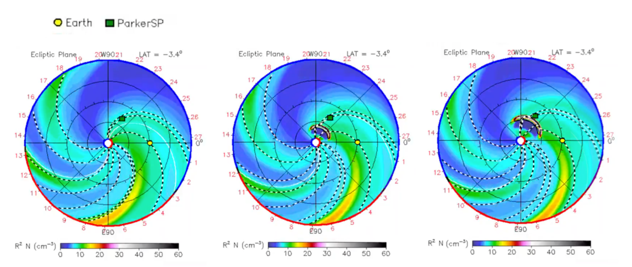
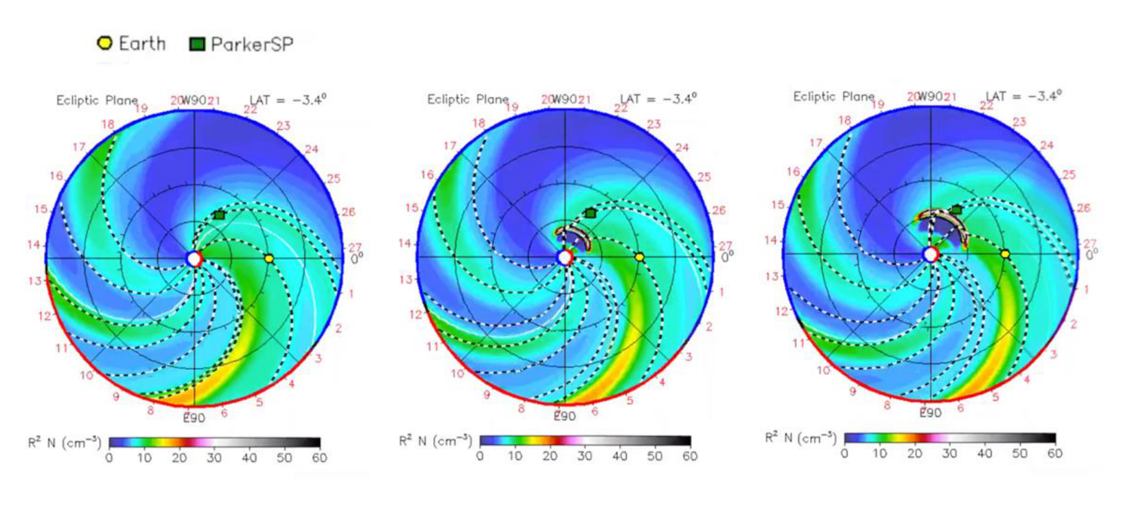
Just recently, on May 28, 2021, a C-shaped CME was detected by the solar space telescope SOHO (located at a distance of km from Earth, around the Sun-Earth L1 Lagrange point) by means of the onboard LASCO coronographs. The solar eruption generating the CME occurred at 22:19 UTC with an ecliptic traveling angle of 55º (with respect to the Sun-Earth line), heading directly towards the point where ParkerSP was located. Figure 1 shows a sequence of three consecutive images made by NASA, highlighting the evolution of the CME, from the onset to the moment it reaches the ParkerSP.
Assume that all spacecrafts are exactly on the ecliptic plane and the images here show a top view of the ecliptic plane.
Part 1 (30 т.)
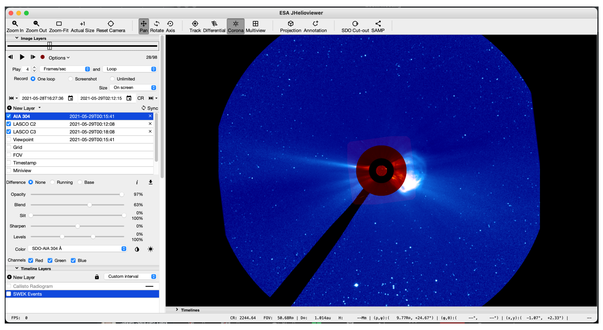
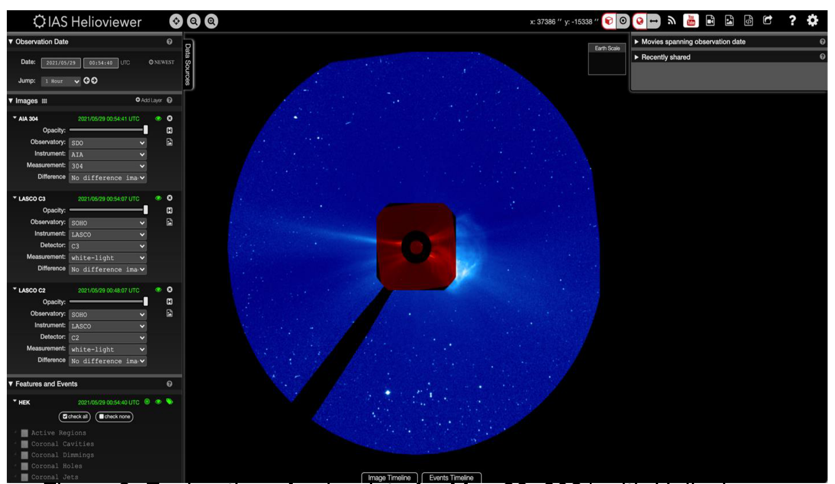
1.1 Using the JHelioviewer software find the CME which occurred on May 28, 2021, by selecting images from the Solar Dynamics Observatory (full disk) and the SOHO-spacecraft coronographs LASCO-C2 (imaging from 2 to 6 solar radii) and LASCO-C3 (imaging from 3.7 to 30 solar radii), as shown in Figure 2. Indicate, in a table, the date and time of each image that you have used. [10 т.]
1.2 Use a selection of images to measure the distance of the CME front from the Sun in km. [10 т.]
1.3 Extend the table of data (that you constructed in previous part) to include
- Date and time (as reported in 1.1)
- Distance of CME front from the Sun in km (as reported in 1.2)
- Cumulative velocity in km/s (e.g. if you are at the 4th image, the mean velocity between onset of CME until the time of the 4th image),
- Velocity per time interval in km/s (e.g if you are at the 4th image, the mean velocity of CME between the times of the 3rd and 4th image).
Make this table in the working sheet. [10 т.]
Note: Both the velocities are to be calculated with respect to the Sun.
Do not forget to label each of the columns of your table accordingly.
Part 2 (15 т.)
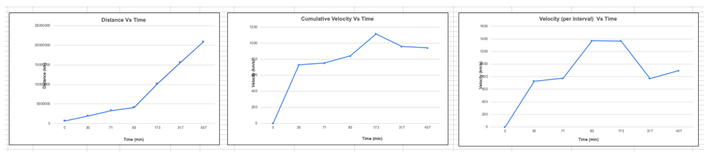
2.1 Make distance-time and velocity-time graphs (for both cumulative and velocity per time interval) using the measured and calculated data from your table. [15 т.]
Part 3 (10 т.)
3.1 Considering that the CME moves at constant speed for distances larger than 30 solar radii, estimate the velocity (in km/s) of the CME front when it impacts the ParkerSP, and the time (in hours) it takes to do so from its onset. [10 т.]
Part 4 (10 т.)
From the following statements, mark which are TRUE and which are FALSE.
4.1 If we keep decreasing the time interval between successive images, the precision of measurements of the evolution of the CME and the calculated physical parameters will always keep increasing. [2 т.]
4.2 A more accurate analysis and measurements of the CME evolution should consider the differential rotation of the Sun, and therefore the calculated velocities will be affected. [2 т.]
4.3 Any software (numerical) misalignment among the images when creating the mosaic will have direct effects on the precision of the calculations. [2 т.]
4.4 The different assumptions made in order to construct the model displayed in a heliospheric density map in Figure 1, may affect the estimation of the Sun-ParkerSP distance. [2 т.]
4.5 The interaction of the CME-front with the remnant dust left by the 2019 Borisov comet broadens and diffuses the images. This reduces the contrast in the images, substantially increasing the uncertainty in determining the CME-front and its propagation. [2 т.]
Part 5 (10 т.)
5.1 The CME front carries a large number of protons and alpha particles. Calculate the energy (in eV) of a single proton and a single alpha particle as measured by the Solar Wind Electrons Alphas and Protons (SWEAP) instrument on board the ParkerSP. Consider only the mechanical energy of the particles resulting from the propagation of the CME front, neglecting all other forms of energy. [10 т.]
Tools
The JHelioviewer software (https://www.jhelioviewer.org/download.html) can be used to explore solar data from several solar telescopes as shown in Figure 2. Using the graphic interface, you can select an observing data (Observation Date) and upload multiple solar images by adding layers (AddLayer). Using the option, you can inspect a sequence of images to study the evolution of an eruptive event. By moving the cursor you get the information about the coordinates where you are located (in arcseconds) with respect to the center of the Sun (x:0” y:0”).
Отговори
Part 3, 3.1 895 km/s; 49.7 hours
From the official solution: velocity of the last interval 895 km/s; total time 7.3 + 42.4 = 49.7 hours.
Part 4, 4.1 FALSE
Part 4, 4.2 FALSE
Part 4, 4.3 TRUE
Part 4, 4.4 FALSE
Part 4, 4.5 FALSE
Part 5, 5.1 Proton: 4181.2 eV; alpha particle: 16598.7 eV
Решение
Part 1
Section 1.1
Data selection (selecting appropriate images showing the evolution of the CME) and identification of CME front.
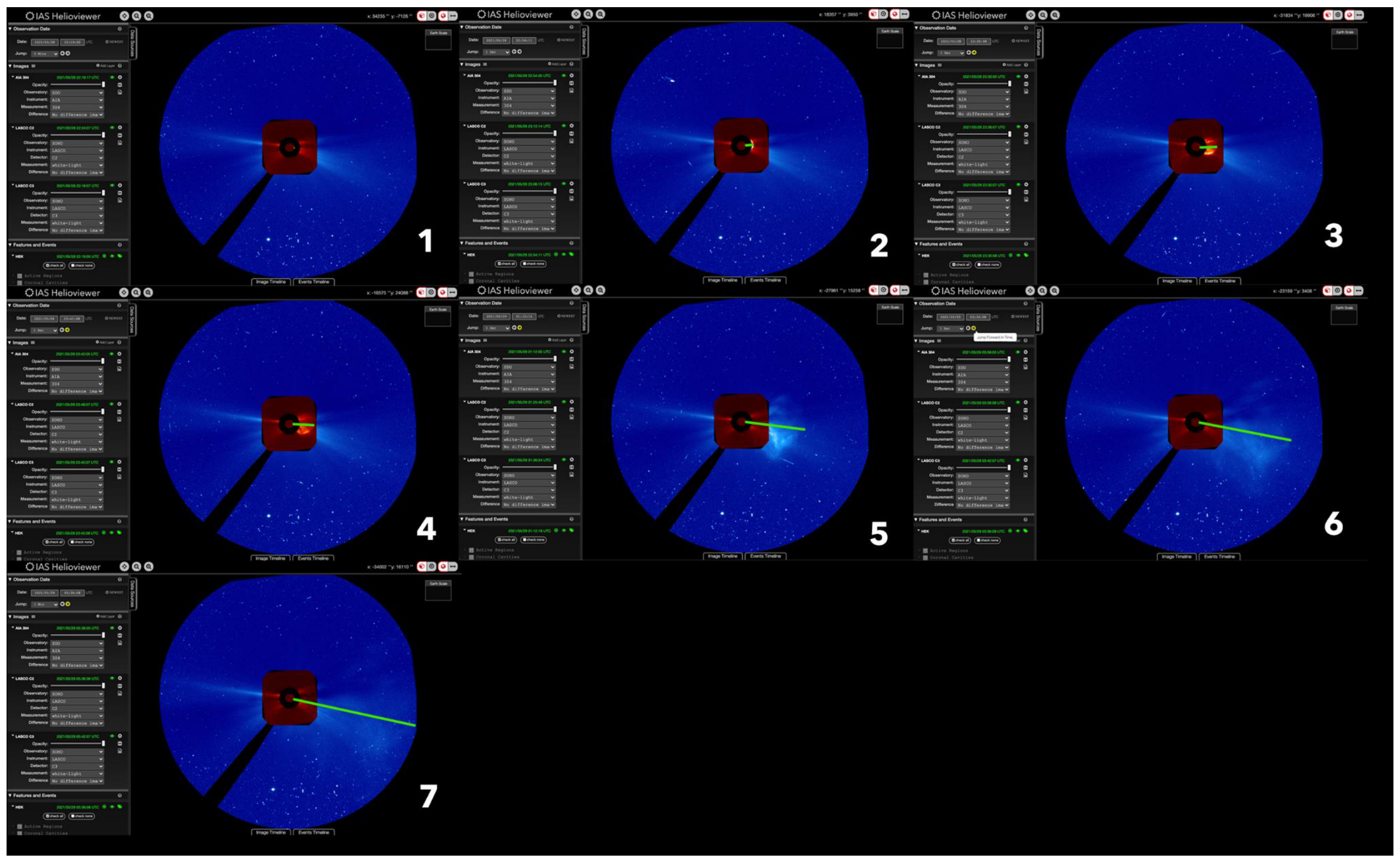
A total of 7 time intervals are selected tracing the evolution of the CME
- 2021/05/28 22:19:00 UT
- 2021/05/28 22:54:11 UT
- 2021/05/28 23:30:08 UT
- 2021/05/29 23:42:08 UT
- 2021/05/29 01:12:16 UT
- 2021/05/29 03:36:08 UT
- 2021/05/29 05:00:08 UT
Section 1.2 and 1.3
Summary of the information extracted from the images for all different selected intervals
| Interval | Date and Time | Time interval (minutes) | Time from CME onset (minutes) | Coordinates of the CME front x" | Coordinates of the CME front y" | Distance from disc center (arcsec) | Distance from disc center (km) | Distance from onset (km) | Cumulative velocity plane of the sky (km/s) | Deprojection of velociity towards ParkerSP (km/s) | Distance per time interval (km) | Velocity on plane of he sky (km/s) | Deprojection of velocity towards ParkerSP (km/s) |
|---|---|---|---|---|---|---|---|---|---|---|---|---|---|
| 1 | 2021/05/28 22:19:00 UT | 0 | 0 | 950 | 144 | 961 | 696617 | 0 | 0 | 0 | 0 | 0 | 0 |
| 2 | 2021/05/28 22:54:11 UT | 35 | 35 | 2682 | 174 | 2688 | 1948538 | 1252198 | 596 | 728 | 1252198 | 596 | 728 |
| 3 | 2021/05/28 23:30:08 UT | 36 | 71 | 4579 | 97 | 4580 | 3320520 | 2624180 | 616 | 752 | 1371982 | 635 | 775 |
| 4 | 2021/05/28 23:42:08 UT | 12 | 83 | 5693 | 116 | 5694 | 4128282 | 3431942 | 689 | 841 | 807762 | 1122 | 1369 |
| 5 | 2021/05/29 01:12:16 UT | 90 | 173 | 14000 | -891 | 14028 | 10170535 | 9474195 | 913 | 1114 | 6042253 | 1119 | 1366 |
| 6 | 2021/05/29 03:36:08 UT | 144 | 317 | 21048 | -4570 | 21538 | 15615349 | 14919009 | 784 | 958 | 5444814 | 630 | 769 |
| 7 | 2021/05/29 05:36:08 UT | 120 | 437 | 27922 | -7126 | 28817 | 20892306 | 20195966 | 770 | 940 | 5276957 | 733 | 895 |
Part 2
Plots: distance vs time and velocity vs time constructed from the information from the previous table.
Part 3
Calculating the velocity of the CME front reaching ParkerSP
The velocity corresponding to the last interval (up to reaching 30 solar radii) is 895 km/s which, according to the considerations of the problem, would be the same velocity of the CME front once it reaches the ParkerSP.
Calculating the time spent by the CME front to reach the ParkerSP from it’s onset.
The Sun-ParkerSP distance estimated from Figure 1 is approx. 0.66 AU = 9.9×10 km = 141 solar radii (given the information that 10 solar radii es approx. 7×10 km)
From the previous analysis, it is known that the CME front reaches a distance of 30 solar radii after 437 minutes (7.3 hours) from its onset (see Table). The distance that the CME travels at the constant speed of 895 km/s is expressed as 141-30=111 solar radii = 7.8x 10 km, and thus the time spent in that interval is 42.4 hours.
Finally, the total time it takes for the CME front to reach the ParkerSP from its onset is computed as: 7.3+ 42.4 = 49.7 hours.
Part 4
True and false statements
If we keep decreasing the time interval between successive images, the precision of measurements of the evolution of the CME and the calculated physical parameters will always keep increasing. FALSE
B. The analysis and measurements of the CME evolution should consider the differential rotation of the Sun, and therefore the calculated velocities will be affected. FALSE
C. Any software (numerical) misalignment among the images when creating the mosaic will have direct effects on the precision of your calculations. TRUE
D. The different assumptions made in order to construct the model displaying in a heliospheric density map in Figure 1, may affect the estimation of the Sun-ParkerSP distance. FALSE
E. The interaction of the CME-front with the remnant dust left by the 2019 Borisov comet broadens and difuminate the images. This substantially intensifies the lack of contrast in the images, increasing the uncertainty in determining the CME-front and its propagation. FALSE
Part 5
Kinetic energy calculations
Proton:
0.5 * (1.67262x10 kg) * (895 km/s) = 4181.2 eV
Alpha particle:
0.5 * (6.64x10 kg) * (895 km/s) = 16598.7 eV
Marking scheme
75 points
Section 1.1
Give A TOTAL number of points following the possible situations (select only one option):
1 points: If the table includes information extracted from a single image (1 frame) for date/time and the corresponding size of the CME (distance measured from the solar limb to the CME front).
2 points: If the table includes information extracted from two images (2 frames) for date/time and the corresponding size of the CME (distance measured from the solar limb to the CME front).
3 points: If the table includes information extracted from three images (3 frames) for date/time and the corresponding size of the CME (distance measured from the solar limb to the CME front).
4 points: If the table includes information extracted from four images (4 frames) for date/time and the corresponding size of the CME (distance measured from the solar limb to the CME front).
5 points: If the table includes information extracted from five of more images (5 or more frames) for date/time and the corresponding size of the CME (distance measured from the solar limb to the CME front).
Section 1.2.
5 points. Values of distance for the number of images used.
5 points: Values of distance in km
Section 1.3
5 points: For calculating the cumulative velocity over the tabulated data
5 points: For calculating the instantaneous velocity (in every time interval) over the tabulated data.
5 points: For considering the deprojection of velocities (from the plane of the sky into the direction towards the location of the ParkerSP).
Part 2
5 points: Plotting the distance vs time for the tabulated data
5 points: Plotting the cumulative velocity vs time.
5 points: Plotting the velocities for all the different time intervals vs time.
Part 3
Velocity and time of CME front
5 points: Estimating the distance (in km) from the Sun to the ParkerSP based on Figure 1 and the appropriate unit conversions.
3 points: Considering the velocity computed for the last interval (up to 30 solar radii) that should be around 800-1000 km/s, as the velocity that impacts the ParkerSP.
2 points: Calculating the time it takes for the CME front to reach the ParkerSP from its onset (in hours), considering the time spend in the first 30 solar radii besides the time the CME is moving at constant speed (from 30 solar radii to the location of the ParkerSP).
Part 4
2 points A. FALSE
2 points B. FALSE
2 points C. TRUE
2 points D.FALSE
2 points E. FALSE
Part 5
4 points. Proton calculation
6 points. Alpha particle calculation
Considerations
Dear team leaders
As some of your teams experienced several troubles when fetching the images that were needed for the observational problem in solar physics, and considering the situation was completely out of our control and that was surely related to the capability of the severs and repositories where the data is stored and accessed, from either JHelioviewer or the web-based Helioviewer tools, we need to contemplate the situation to slightly adjust the evaluation process accordingly.
We aim at having all participants being evaluated under the same conditions, but in a few cases, and after not being able to get the images from the platform, we decided to provide a set of images for them to be able to start solving the questions. For this reason, the Academic Committee, for the sake of maintaining the fair principles of the Olympiads that we all promote among our teams, considers that the observational problem has to evaluate primarily the measurements that students have done over the set of images tracking the evolution of the solar CME, giving less weight to the initial part of purely selecting images.
Nonetheless, those students which spent time fetching images should receive at least some points, which won’t represent a significant part of the grading, that will compensate the effort they have done for getting their set of images to start with.
In summary, we propose section 1.1 to receive 5 points (instead of 10) and section 1.2 to increase from 10 points to 15 points (being the most important part to evaluate the measurements made by the students). Section 1.3 keeps 10 points.
1.1 Using the JHelioviewer software find the CME which occurred on May 28, 2021, by using images from the Solar Dynamics Observatory (full disk) and the SOHO- spacecraft coronographs LASCO-C2 (imaging from 2 to 6 solar radii) and LASCO-C3 (imaging from 3.7 to 30 solar radii), as shown in Figure 2. [5 points]
1.2 Use a selection of images to measure the distance of the CME front from the Sun, and derive its velocity over time [10 points]
1.3 Use these values to construct a table, dividing it in two parts (left and right). • The first part of the table (left) should contain your measurements characterizing every image (including date/time). • The second part (right) should have your calculations: distance, cumulative velocity, and velocity per time interval (depending on the number of images you are employing, for instance from first to second image, second to third, etc.). [15 points]
Earlier question version printed with the solution
Solar Physics: Observational data analysis
Proposed by: Juan Camilo Buitrago and Santiago Vargas
75 points
The solar slap [75 points]
Solar Cycle 25 is heating up! It began in December 2019 and will peak in 2025. The start of a new cycle means there will be increasing solar activity until roughly mid-2025. One direct consequence of such activity is the more frequent occurrence of solar flares, which are intense bursts of radiation observed near the Sun’s photosphere and low-corona. Solar flares are sometimes accompanied by coronal mass ejections (CMEs), which expel coronal plasma into the interplanetary space.
We are living in a golden age for solar astrophysics. In addition to entering a period of high solar activity, we also have brand new cutting-edge solar telescopes that will allow us to study the Sun as never before. One of these telescopes is the Parker Solar Probe (ParkerSP), the first spacecraft in history to fly into the low solar corona. The ParkerSP has a somewhat eccentric orbit (ε≈0.88) and will approach the Sun as close as 7 million km (10 solar radii) on its final orbital perihelium (in 2025). Just recently, on May 28, 2021, a C-shaped CME was detected by the NASA solar space telescope SOHO (located at a distance of 1.5 x 10 km from Earth, around the Sun-Earth L1 Lagrange point) by means of the onboard LASCO coronographs. The solar eruption generating the CME occurred at 22:19 UTC with an ecliptic traveling angle of 55º (respect to the Sun-Earth line), heading directly towards the point where ParkerSP was located. Figure 1 shows a sequence of three consecutive images made by the NASA Community Coordinated Modeling Center, highlighting the evolution of the CME for three moments, from the onset to the moment it reaches the ParkerSP.
[30 points]
- Using the JHelioviewer find the CME which occurred on May 28, 2021, by using images from the Solar Dynamics Observatory (full disk) and the SOHO-spacecraft coronographs LASCO-C2 (imaging from 1.5 to 6 solar radii) and LASCO-C3 (imaging from 3.7 to 30 solar radii), as shown in Figure 2.
- Use a selection of images to measure the distance of the CME-front from the Sun, and derive its velocity over time.
- Use these values to construct a table dividing it in two parts (left and right). i. The first part of the table (left) should contain your measurements characterizing every image (including date/time).
ii. The second part (right) should have your calculations: distance, cumulative velocity, and velocity per time interval (depending on the number of images you are employing, for instance from first to second image, second to third, etc.). - Do not forget to label each of the columns of your table accordingly.
[15 points] Make distance-time and velocity-time graphs using the measured and calculated data from your table.
[10 points] Considering that the CME moves at constant speed for distances larger than 30 solar radii, estimate the velocity (in km/s) of the CME front when it impacts the ParkerSP, and the time (in hours) it takes to do so from its onset.
[10 points] From the following statements, select the ones which are TRUE and the ones which are FALSE.
A. A larger number of selected images would give more precise information on the evolution of the CME and the calculated physical parameters.
B. A more precise analysis and measurements of the CME evolution should consider the differential rotation of the Sun, and therefore the calculated velocities will be affected.
C. Any software (numerical) misalignment among the images when creating the mosaic will have direct effects on the precision of the calculations.
D. The different assumptions made in order to construct the model displaying in a heliospheric density map in Figure 1, may affect the estimation of the Sun-ParkerSP distance.
E. The interaction of the CME-front with the remnant dust left by the 2019 Borisov comet broadens and difuminate the images. This intensifies the lack of contrast in the images, increasing the uncertainty in determining the CME-front and its propagation.[10 points] Knowing that the CME front carries a large population of protons and alpha particles, compute the expected energy (in eV) measured for a single of these types of particles, by the Solar Wind Electrons Alphas and Protons (SWEAP) instrument onboard the ParkerSP. Neglect the rest mass energy of each particle and consider the proton mass to be 1.67262 x 10 kg.
Tools The JHelioviewer software (https://www.jhelioviewer.org/download.html) can be used to explore solar data from several solar telescopes as shown in Figure 2. Using the graphic interface you can select an observing data (Observation Date) and upload multiple solar images by adding layers (AddLayer). Using the option Jump, you can inspect a sequence of images to study the evolution of an eruptive event. By moving the cursor you get the information about the coordinates where you are located (in arcseconds) with respect to the center of the Sun (x:0” y:0”).
Оригинал в Архива: Observational Solar Physics Problems.pdf · официални решения: Observational Solar Physics Solutions.pdf