Съдържание

Условие Available equipment Отговори Решение Page n. 1 Page n. 2 Page n. 3 Page n. 4

IPhO 1999, Експеримент — Задача 1. Torsion pendulum

Оригинал на условието (PDF)Съобщи за грешка

Всички материали от IPhO 1999

30th International Physics Olympiad, Padua, Italy — Experimental competition · 20 юли 1999 г.

Внимание: Бележка към темата

И двете архивни копия съдържат 7 страници условие и 7 страници официално решение. На първата страница на условието е посочен комплект от 11 страници, включващ бланките за отговор. Четирите бланки липсват в двете английски архивни копия. Официалният италиански вариант съдържа четирите бланки за същия експеримент. Те са номерирани 1–4 и се намират на страници 8–12 от преобразувания в PDF италиански източник; страница 13 повтаря само заглавната част на последната бланка. Всичките осем задачи и наличното решение са запазени в една обща задача. В таблицата към задачи 5–6 оригиналът отпечатва единица N·µm, а фигура 8 използва N·mm; и двете означения са запазени. Числените резултати в решението са от предварителен пробен опит и са дадени само като ориентир.

Please read this first:

Before attempting to assemble your equipment, read the problem text completely!

The time available is 5 hours for one experiment only.
Use only the pen provided.
Use only the front side of the provided sheets.
In addition to "blank" sheets where you may write freely, there is a set of Answer sheets where you must summarize the results you have obtained. Numerical results must be written with as many digits as appropriate; don’t forget the units. Try – whenever possible – to estimate the experimental uncertainties.
Please write on the "blank" sheets the results of all your measurements and whatever else you deem important for the solution of the problem, that you wish to be evaluated during the marking process. However, you should use mainly equations, numbers, symbols, graphs, figures, and use as little text as possible.
It's absolutely imperative that you write on top of each sheet that you'll use: your name (“NAME”), your country (“TEAM”), your student code (as shown on your identification tag, “CODE”), and additionally on the "blank" sheets: the progressive number of each sheet (from 1 to $N$ , “Page n.”) and the total number ( $N$ ) of "blank" sheets that you use and wish to be evaluated (“Page total”); leave the “Problem” field blank. It is also useful to write the number of the section you are answering at the beginning of each such section. If you use some sheets for notes that you don’t wish to be evaluated by the marking team, just put a large cross through the whole sheet, and don’t number it.
When you've finished, turn in all sheets in proper order (answer sheets first, then used sheets in order, unused sheets and problem text at the bottom) and put them all inside the envelope where you found them; then leave everything on your desk. You are not allowed to take anything out of the room.

This problem consists of 11 pages (including this one and the answer sheets).

This problem has been prepared by the Scientific Committee of the 30th IPhO, including professors at the Universities of Bologna, Naples, Turin and Trieste.

Условие

In this experiment we want to study a relatively complex mechanical system – a torsion pendulum – and investigate its main parameters. When its rotation axis is horizontal it displays a simple example of bifurcation.

Available equipment

A torsion pendulum, consisting of an outer body (not longitudinally uniform) and an inner threaded rod, with a stand as shown in figure 1
A steel wire with handle
A long hexagonal nut that can be screwed onto the pendulum threaded rod (needed only for the last exercise)
A ruler and a right triangle template
A timer
Hexagonal wrenches
A3 Millimeter paper sheets.
An adjustable clamp
Adhesive tape
A piece of T-shaped rod

The experimental apparatus is shown in figure 1; it is a torsion pendulum that can oscillate either around a horizontal rotation axis or around a vertical rotation axis. The rotation axis is defined by a short steel wire kept in tension. The pendulum has an inner part that is a threaded rod that may be screwed in and out, and can be fixed in place by means of a small hexagonal lock nut. This threaded rod can not be extracted from the pendulum body.

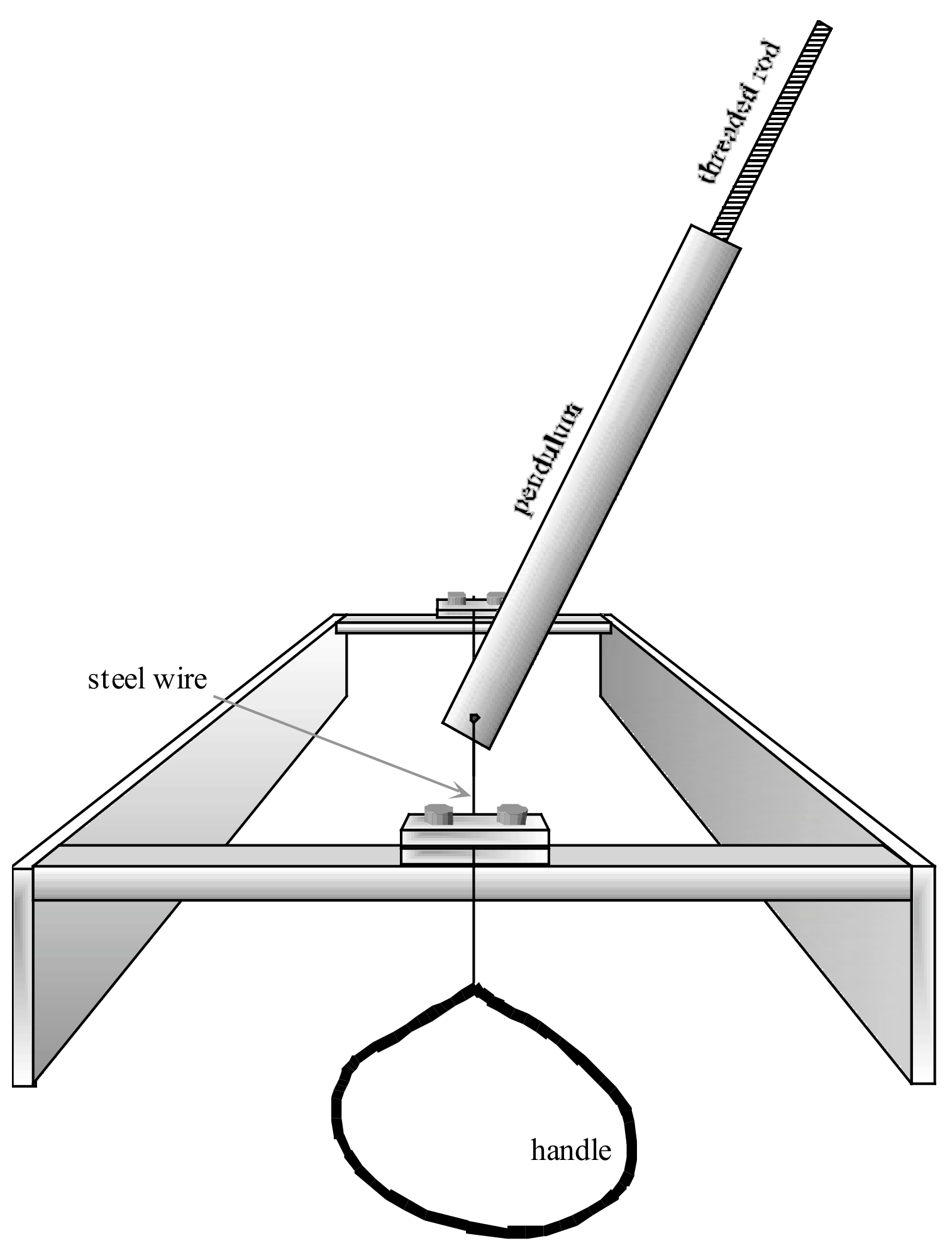
Perspective sketch of the apparatus: a stand frame with two sloping side brackets and a horizontal cross bar; a steel wire runs between two clamping blocks with screws, and below the stand it ends in a loop labelled 'handle'; the pendulum, a long cylinder labelled 'pendulum', is attached to the wire and tilted, with a threaded rod labelled 'threaded rod' sticking out of its upper end; an arrow labels the 'steel wire'. — Figure 1: Sketch of the experimental apparatus when its rotation axis is horizontal.

When assembling the apparatus in step 5 the steel wire must pass through the brass blocks and through the hole in the pendulum, then must be locked in place by keeping it stretched: lock it first at one end, then use the handle to put it in tension and lock it at the other end.

Warning: The wire must be put in tension only to guarantee the pendulum stability. It's not necessary to strain it with a force larger than about 30 N. While straining it, don't bend the wire against the stand, because it might break.

The variables characterizing the pendulum oscillations are:

the pendulum position defined by the angle $\theta$ of deviation from the direction perpendicular to the plane of the stand frame, which is shown horizontal in figure 1.
the distance $x$ between the free end of the inner threaded rod and the pendulum rotation axis
the period $T$ of the pendulum oscillations.

The parameters characterizing the system are:

the torsional elastic constant $\kappa$ (torque = $\kappa \cdot$ angle) of the steel wire;
the masses $M_1$ and $M_2$ of the two parts of the pendulum (1: outer cylinder $^{1}$ and 2: threaded rod);
the distances $R_1$ and $R_2$ of the center of mass of each pendulum part (1: outer cylinder and 2: threaded rod) from the rotation axis. In this case the inner mobile part (the threaded rod) is sufficiently uniform for computing $R_2$ on the basis of its mass, its length $\ell$ and the distance $x$ . $R_2$ is therefore a simple function of the other parameters;
the moments of inertia $I_1$ and $I_2$ of the two pendulum parts (1: outer cylinder and 2: threaded rod). In this case also we assume that the mobile part (the threaded rod) is sufficiently uniform for computing $I_2$ on the basis of its mass, its length $\ell$ and the distance $x$ . $I_2$ is therefore also a simple function of the other parameters;
the angular position $\theta_0$ (measured between the pendulum and the perpendicular to the plane of the stand frame) where the elastic recall torque is zero. The pendulum is locked to the rotation axis by means of a hex screw, opposite to the threaded rod; therefore $\theta_0$ varies with each installation of the apparatus.

$^{1}$ Including the small hex locking nut.

Summing up, the system is described by 7 parameters: $\kappa$ , $M_1$ , $M_2$ , $R_1$ , $I_1$ , $\ell$ , $\theta_0$ , but $\theta_0$ changes each time the apparatus is assembled, so that only 6 of them are really constants and the purpose of the experiment is that of determining them, namely $\kappa$ , $M_1$ , $M_2$ , $R_1$ , $I_1$ , $\ell$ , experimentally. Please note that the inner threaded rod can’t be drawn out of the pendulum body, and initially only the total mass $M_1 + M_2$ is given (it is printed on each pendulum).

In this experiment several quantities are linear functions of one variable, and you must estimate the parameters of these linear functions. You can use a linear fit, but alternative approaches are also acceptable. The experimental uncertainties of the parameters can be estimated from the procedure of the linear fit or from the spread of experimental data about the fit.

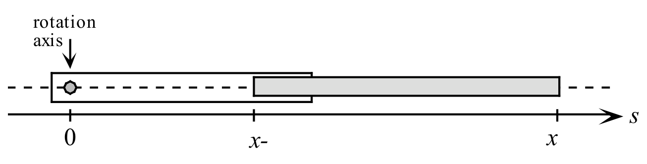
The analysis also requires a simple formula for the moment of inertia of the inner part (we assume that its transverse dimensions are negligible with respect to its length, see figure 2):

I_2(x) = \int_{x-\ell}^{x} \lambda\, s^2 ds = \frac{\lambda}{3}\left(x^3 - (x-\ell)^3\right) = \frac{\lambda}{3}\left(3\ell x^2 - 3\ell^2 x + \ell^3\right) \qquad (1)

where $\lambda = M_2/\ell$ is the linear mass density, and therefore

I_2(x) = M_2 x^2 - M_2 \ell x + \frac{M_2}{3}\ell^2 \qquad (2)

Schematic along an s axis: an outer rectangular body with a small circle marking the rotation axis (arrow labelled 'rotation axis') at s = 0, and a shaded inner bar extending from the tick labelled x- to the tick labelled x. — Figure 2: In the analysis of the experiment we can use an equation (eq. 2) for the moment of inertia of a bar whose transverse dimensions are much less than its length. The moment of inertia must be computed about the rotation axis that in this figure crosses the $s$ axis at $s$ =0.

Now follow these steps to find the 6 parameters $M_1$ , $M_2$ , $\kappa$ , $R_1$ , $\ell$ , $I_1$ :

1. The value of the total mass $M_1+M_2$ is given (it is printed on the pendulum), and you can find $M_1$ and $M_2$ by measuring the distance $R(x)$ between the rotation axis and the center of mass of the pendulum. To accomplish this write first an equation for the position $R(x)$ of the center of mass as a function of $x$ and of the parameters $M_1$ , $M_2$ , $R_1$ , $\ell$ . [0,5 т.]

2. Now measure $R(x)$ for several values of $x$ (at least 3) $^{2}$ . Clearly such measurement must be carried out when the pendulum is not attached to the steel wire. Use these measurements and the previous result to find $M_1$ and $M_2$ .

$^{2}$ The small hex nut must be locked in place every time you move the threaded rod. Its mass is included in $M_1$ . This locking must be repeated also in the following, each time you move the threaded rod. [3 т.]

3. Find an equation for the pendulum total moment of inertia $I$ as a function of $x$ and of the parameters $M_2$ , $I_1$ and $\ell$ . [0,5 т.]

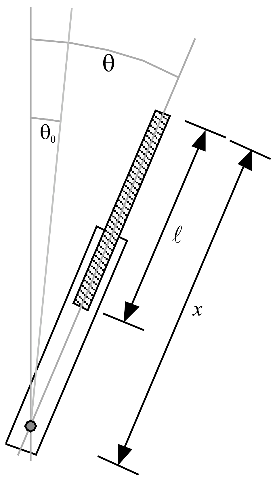
4. Write the pendulum equation of motion in the case of a horizontal rotation axis, as a function of the angle $\theta$ (see figure 3) and of $x$ , $\kappa$ , $\theta_0$ , $M_1$ , $M_2$ , the total moment of inertia $I$ and the position $R(x)$ of the center of mass.

The pendulum drawn tilted from the vertical: a vertical grey line through the rotation axis, a grey line at angle θ0 marking the zero-torque position, and the pendulum axis at angle θ; a hatched threaded rod sticks out of the outer body; dimension arrows mark the rod length ℓ and the distance x from the rotation axis to the free end of the rod. — Figure 3: The variables $\theta$ and $x$ and the parameters $\theta_0$ and $\ell$ are shown here.

[1 т.]

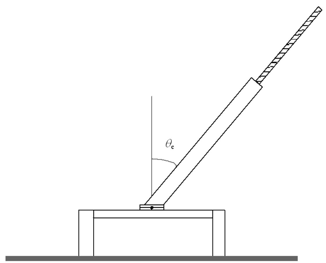
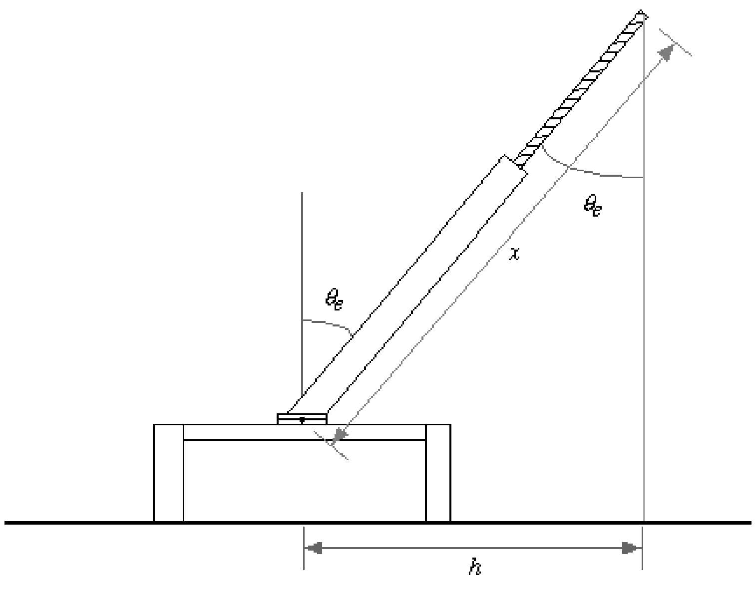
5. In order to determine $\kappa$ , assemble now the pendulum and set it with its rotation axis horizontal. The threaded rod must initially be as far as possible inside the pendulum. Lock the pendulum to the steel wire, with the hex screw, at about half way between the wire clamps and in such a way that its equilibrium angle (under the combined action of weight and elastic recall) deviates sizeably from the vertical (see figure 4). Measure the equilibrium angle $\theta_e$ for several values of $x$ (at least 5).

Side view of the stand on a table with the pendulum and its threaded rod tilted from the vertical line by the equilibrium angle θe. — Figure 4: In this measurement set the pendulum so that its equilibrium position deviates from the vertical.

[4 т.]

6. Using the last measurements, find $\kappa$ . [4,5 т.]

7. Now place the pendulum with its rotation axis vertical $^{3}$ , and measure its oscillation period for several values of $x$ (at least 5). With these measurements, find $I_1$ and $\ell$ .

$^{3}$ In order to stabilize it in this position, you may reposition the stand brackets. [4 т.]

At this stage, after having found the system parameters, set the experimental apparatus as follows:

pendulum rotation axis horizontal
threaded rod as far as possible inside the pendulum
pendulum as vertical as possible near equilibrium
finally add the long hexagonal nut at the end of the threaded rod by screwing it a few turns (it can’t go further than that)

In this way the pendulum may have two equilibrium positions, and the situation varies according to the position of the threaded rod, as you can also see from the generic graph shown in figure 5, of the potential energy as a function of the angle $\theta$ .

The doubling of the potential energy minimum in figure 5 illustrates a phenomenon known in mathematics as bifurcation; it is also related to the various kinds of symmetry breaking that are studied in particle physics and statistical mechanics.

We can now study this bifurcation by measuring the period of the small oscillations about the equilibrium position:

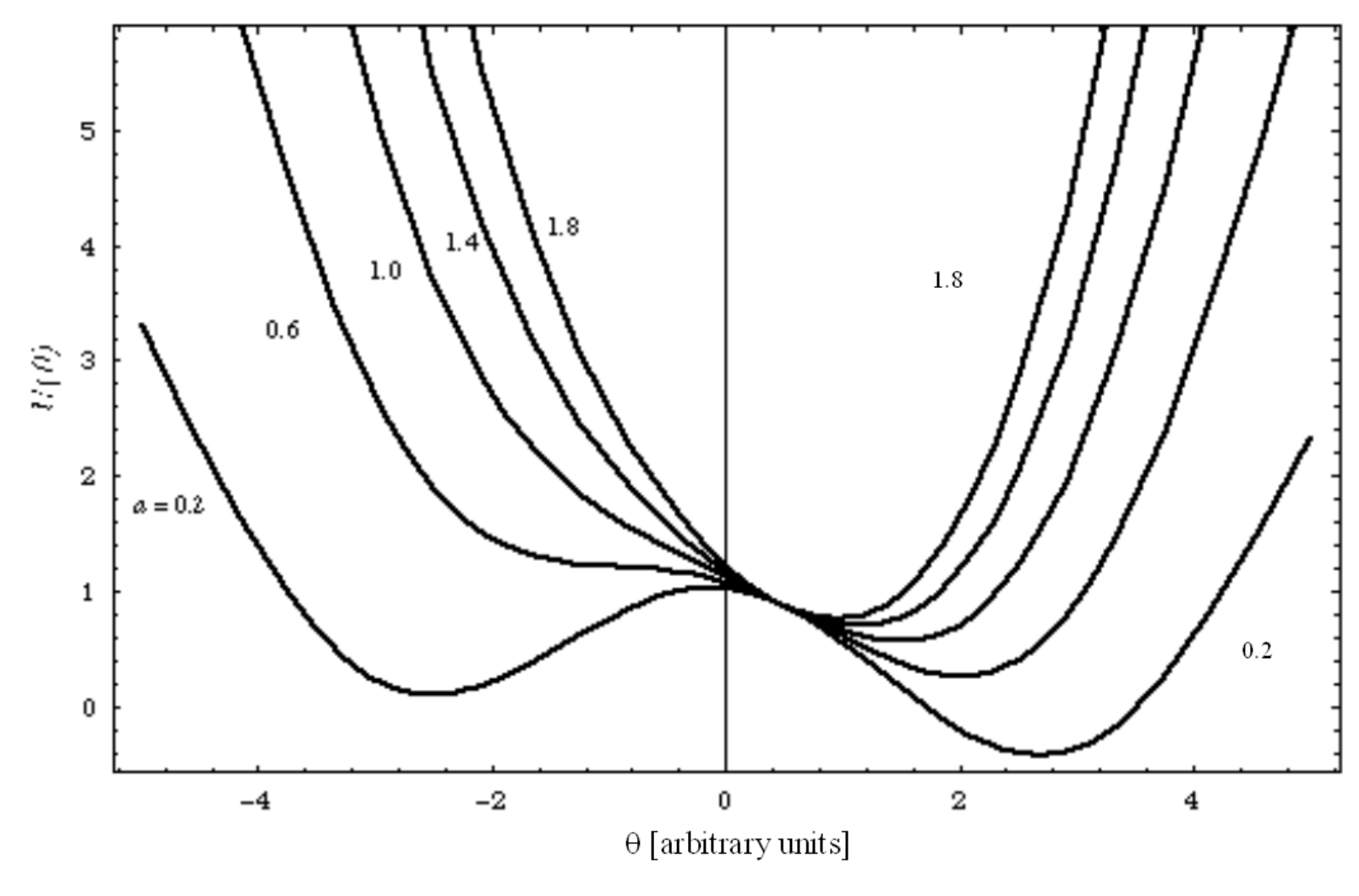
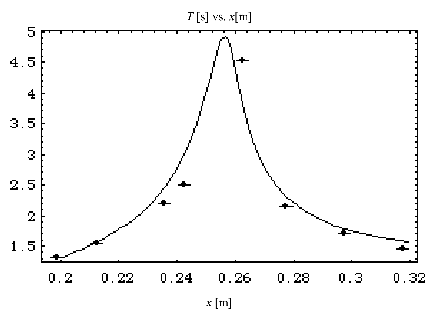
Graph of U(θ) against θ [arbitrary units] from −5 to 5, vertical axis from 0 to 5; curves labelled a = 0.2, 0.6, 1.0, 1.4, 1.8; the curve for a = 0.2 has two minima (near θ ≈ −2.5 and θ ≈ 2.7), while the curves for larger a have a single minimum. — Figure 5: Graph of the function $U(\theta) = \frac{a}{2}(\theta - \theta_0)^2 + \cos\theta$ (which is proportional to the potential energy of this problem) as a function of $\theta$ , with $\theta_0 \neq 0$ . The various curves correspond to different $a$ values as labeled in the figure; smaller values of $a$ ( $a < 1$ ) correspond to the appearance of the bifurcation. In our case the parameter $a$ is associated with the position $x$ of the threaded rod.

8. Plot the period $^{4}$ $T$ as a function of $x$ . What kind of function is it? Is it increasing, decreasing or is it a more complex function?

$^{4}$ You may be able to observe two equilibrium positions, but one of them is more stable than the other (see figure 5). Report and plot the period for the more stable one. [2,5 т.]

Отговори

Решение

The numerical values given in the text are those obtained in a preliminary test performed by a student of the University of Bologna $^{1}$ , and are reported here only as a guide to the evaluation of the student solutions.

$^{1}$ Mr. Maurizio Recchi.

1. and 2.

The distance from the center of mass to the rotation axis is:

R(x) = \frac{M_1 R_1 + M_2 (x - \ell/2)}{M_1 + M_2} \qquad (1)

and therefore, if we measure the position of the center of mass $^{2}$ as a function of $x$ we obtain a relationship between the system parameters, and by a linear fit of eq. (1) we obtain an angular coefficient equal to $M_2/(M_1 + M_2)$ , and from these equations, making use of the given total mass $M_1 + M_2 =$ 41.0 g ± 0.1 g, we obtain $M_1$ and $M_2$ . The following table shows some results obtained in the test run.

$^{2}$ This can easily be done by balancing the pendulum, e.g. on the T-shaped rod provided.

n	x [mm]	R(x) [mm]
1	204±1	76±1
2	220±1	83±1
3	236±1	89±1
4	254±1	95±1
5	269±1	101±1
6	287±1	107±1
7	302±1	113±1
8	321±1	119±1

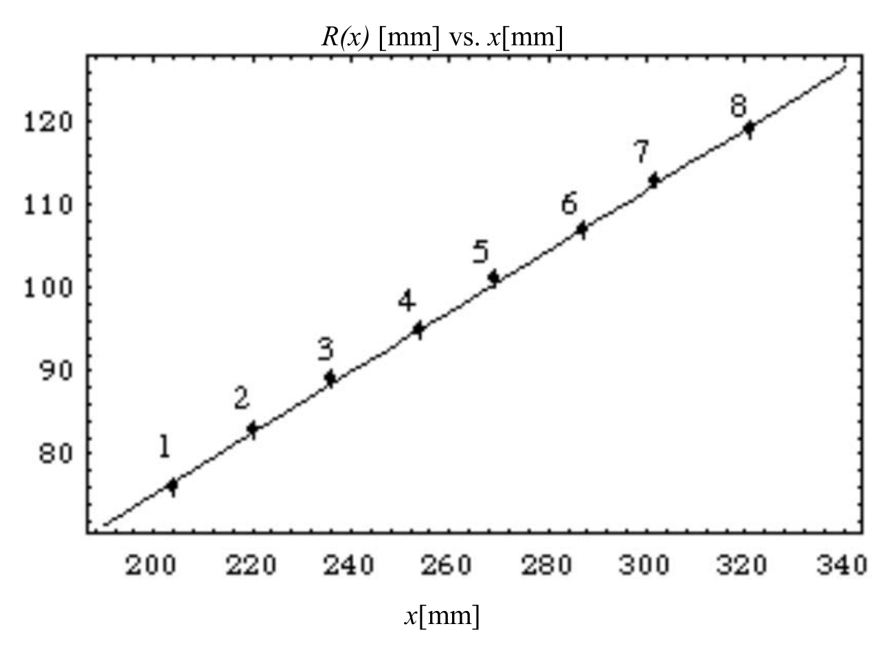
Plot titled 'R(x) [mm] vs. x[mm]': eight data points numbered 1–8 with error bars rising from about 76 mm at x = 204 mm to about 119 mm at x = 321 mm, lying on a best-fit straight line; x axis 200–340, y axis 80–120. — Figure 6: Graph of the position of the pendulum's center of mass (with respect to the rotation axis) as a function of the variable $x$ . The numbering of the data points corresponds to that mentioned in the main text. The estimated error is compatible with the fluctuations of the measured data.

Figure 6 shows the data concerning the position of the pendulum's center of mass together with a best fit straight line: the estimated error on the length measurements is now 1 mm and we treat it as a Gaussian error. Notice that both the dependent variable $R(x)$ and the independent variable $x$ are affected by the experimental uncertainty, however we decide to neglect the uncertainty on $x$ , since it is smaller than 1%. The coefficients $a$ and $b$ in $R(x) = ax+b$ are

$a = 0.366 \pm 0.009$

$b = 2\ \mathrm{mm} \pm 2\ \mathrm{mm}$

(therefore $b$ is compatible with 0)

For computing the masses only the $a$ value is needed; using the total pendulum mass we find:

$M_1 = 26.1 \pm 0.4\ \mathrm{g}$

$M_2 = 15.0\ \mathrm{g} \pm 0.4\ \mathrm{g}$

Even though many non-programmable pocket calculators can carry out a linear regression, it is likely that many students will be unable to do such an analysis, and in particular they may be unable to estimate the uncertainty of the fit parameters even if their pocket calculators provide a linear regression mode. It is also acceptable to find $a$ and $b$ using several pairs of measurements and finally computing a weighted average of the results. For each pair of measurements $a$ and $b$ are given by

a = \frac{y_2 - y_1}{x_2 - x_1}, \qquad b = y_2 - a x_2 \qquad (2)

and the parameter uncertainties (assuming them gaussian) by

\Delta a = a\sqrt{\frac{\Delta x_1^2 + \Delta x_2^2}{(x_1 - x_2)^2} + \frac{\Delta y_1^2 + \Delta y_2^2}{(y_1 - y_2)^2}}, \qquad \Delta b = \sqrt{\Delta y_2^2 + a^2 x_2^2 \left(\frac{\Delta x_2^2}{x_2^2} + \frac{\Delta a^2}{a^2}\right)} \qquad (3)

In order to calculate (2) and (3) the data can be paired with a scheme like $\{1,5\},\{2,6\},\{3,7\},\{4,8\}$ , where "far" points are coupled in order to minimize the error on each pair.

There may be other alternative and equally acceptable approaches: they should all be considered valid if the order of magnitude of the estimated uncertainty is correct.

3.

The pendulum's total moment of inertia is the sum of the moments of its two parts, and from figure 3 we see that

I(x) = I_1 + I_2(x) = M_2 x^2 - M_2 \ell x + \left(I_1 + \frac{M_2}{3}\ell^2\right) \qquad (4)

4.

The pendulum's equation of motion is

I(x)\frac{d^2\theta}{dt^2} = -\kappa(\theta - \theta_0) \qquad (5)

if the rotation axis is vertical, while it's

I(x)\frac{d^2\theta}{dt^2} = -\kappa(\theta - \theta_0) + (M_1 + M_2) g R(x) sin\theta \qquad (6)

if the rotation axis is horizontal.

5. and 6.

When the system is at rest in an equilibrium position, the angular acceleration is zero and therefore the equilibrium positions $\theta_e$ can be found by solving the equation

-\kappa(\theta_\mathrm{e} - \theta_0) + (M_1 + M_2) g R(x) \sin\theta_\mathrm{e} = 0 \qquad (7)

If the value $x_i$ corresponds to the equilibrium angle $\theta_{e,i}$ , and if we define the quantity (that can be computed from the experimental data) $y_i = (M_1 + M_2) g R(x_i) \sin\theta_{e,i}$ , then eq. (7) may be written as

y_i = \kappa\theta_{e,i} - \kappa\theta_0 \qquad (8)

and therefore the quantities $\kappa$ and $\kappa\theta_0$ can be found with a linear fit. The following table shows several data collected in a trial run according to the geometry shown in figure 7.

Side view of the stand on a table with the pendulum tilted by the equilibrium angle θe from the vertical; the distance x along the pendulum to the free end of the threaded rod is marked, a vertical line drops from the rod end to the table, and the horizontal distance h from the rotation axis to that line is marked; the angle θe is also shown at the rod end. — Figure 7: Geometry of the measurements taken for finding the angle.

n	x [mm]	h [mm]	$\sin\theta_\mathrm{e} = h/x$	$\theta_\mathrm{e}$	y [N·µm]
1	204±1	40±1	0.196±0.005	0.197±0.005	6.1±0.3
2	220±1	62±1	0.282±0.005	0.286±0.005	9.4±0.4
3	238±1	75±1	0.315±0.004	0.321±0.005	11.3±0.5
4	255±1	89±1	0.349±0.004	0.357±0.004	13.4±0.5
5	270±1	109±1	0.404±0.004	0.416±0.004	16.4±0.6
6	286±1	131±1	0.458±0.004	0.476±0.004	19.7±0.7
7	307±1	162±1	0.528±0.004	0.556±0.004	24.3±0.8
8	321±1	188±1	0.586±0.004	0.626±0.004	28.2±0.9

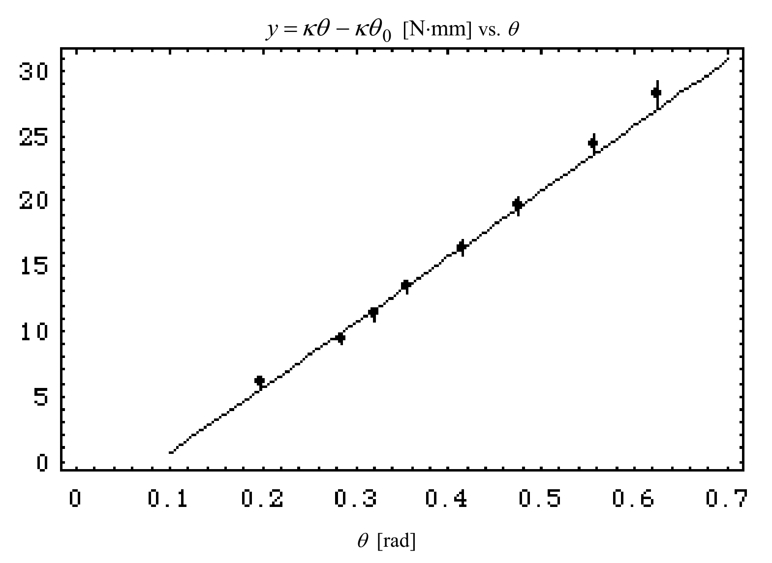
We see that not only the dependent but also the independent variable is affected by a measurement uncertainty, but the relative uncertainty on $\theta_\mathrm{e}$ is much smaller than the relative uncertainty on $y$ and we neglect it. We obtain from such data (neglecting the first data point, see figure 8):

$\kappa = 0.055\ \mathrm{N{\cdot}m{\cdot}rad^{-1}} \pm 0.001\ \mathrm{N{\cdot}m{\cdot}rad^{-1}}$

$\kappa\theta_0 = -0.0063\ \mathrm{N{\cdot}m} \pm 0.0008\ \mathrm{N{\cdot}m}$

Clearly in this case only the determination of the torsion coefficient $\kappa$ is interesting. The fit of the experimental data is shown in figure 8.

Plot titled 'y = κθ − κθ0 [N·mm] vs. θ': eight data points with error bars from about 6 at θ ≈ 0.2 rad to about 28 at θ ≈ 0.63 rad and a fitted straight line; x axis θ [rad] from 0 to 0.7, y axis 0 to 30. — Figure 8: Fit of eq. (8) as a function of $\theta$ . In this case the estimated error is again compatible with the experimental data fluctuations. However the data points show a visible deviation from straightness which may be due to an error in the first measurement (the one at lowest $\theta$ ).

7.

The moment of inertia can be found experimentally using the pendulum with its rotation axis vertical and recalling eq. (5); from this equation we see that the pendulum oscillates with angular frequency $\omega(x) = \sqrt{\dfrac{\kappa}{I(x)}}$ and therefore

I(x) = \frac{\kappa T^2(x)}{4\pi^2} \qquad (9)

where $T$ is the measured oscillation period. Using eq. (9) we see that eq. (4) can be rewritten as

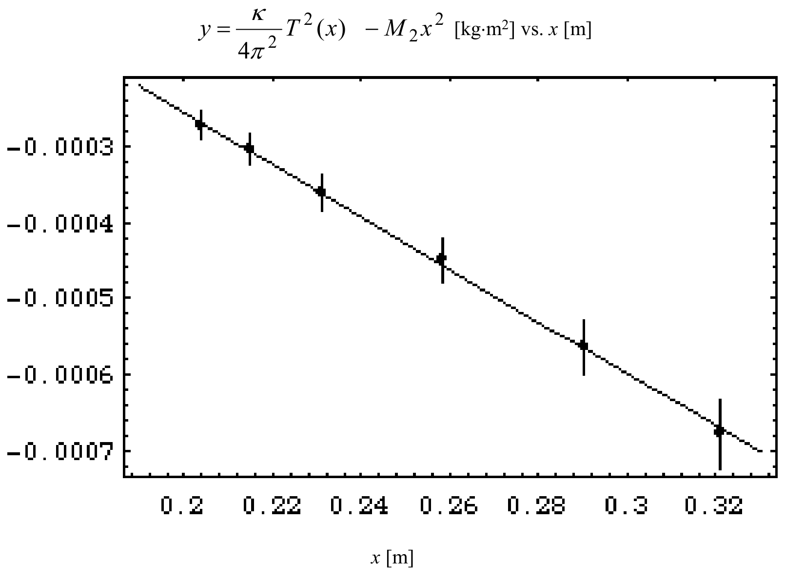
\frac{\kappa}{4\pi^2} T^2(x) - M_2 x^2 = -M_2 \ell x + \left(I_1 + \frac{M_2}{3}\ell^2\right) \qquad (10)

The left-hand side in eq. (10) is known experimentally, and therefore with a simple linear fit we can find the coefficients $M_2 \ell$ and $\left(I_1 + \dfrac{M_2}{3}\ell^2\right)$ , as we did before. The experimental data are in this case:

n	x [mm]	T [s]
1	204±1	0.502±0.002
2	215±1	0.528±0.002
3	231±1	0.562±0.002
4	258±1	0.628±0.002
5	290±1	0.708±0.002
6	321±1	0.790±0.002

The low uncertainty on $T$ has been obtained measuring the total time required for 50 full periods.

Using the previous data and another linear fit, we find

$\ell = 230\ \mathrm{mm} \pm 20\ \mathrm{mm}$

$I_1 = 1.7 \cdot 10^{-4}\ \mathrm{kg{\cdot}m^2} \pm 0.7 \cdot 10^{-4}\ \mathrm{kg{\cdot}m^2}$

and the fit of the experimental data is shown in figure 9.

Plot titled 'y = κT²(x)/(4π²) − M2x² [kg·m²] vs. x [m]': six data points with error bars falling from about −0.00028 at x = 0.204 m to about −0.00067 at x = 0.321 m, on a fitted descending straight line; x axis 0.2–0.32 m, y axis −0.0003 to −0.0007. — Figure 9: Fit of eq. (10) as a function of $x$ . In this case the estimated error is again compatible with the experimental data fluctuations.

8.

Although in this case the period $T$ is a complicated function of $x$ , its graph is simple, and it is shown in figure 10, along with the test experimental data.

The required answer is that there is a single local maximum.

Plot titled 'T [s] vs. x[m]': a theoretical curve rising from about 1.3 s at x = 0.2 m to a sharp peak of about 4.9 s near x ≈ 0.256 m and falling to about 1.6 s at x = 0.32 m, with eight experimental points (e.g. 4.5 s at x ≈ 0.262 m) scattered near it; x axis 0.2–0.32 m, y axis 1.5–5 s. — Figure 10: The period $T$ of the pendulum with horizontal axis as a function of $x$ . In addition to the experimental points the figure shows the result of a theoretical calculation of the period in which the following values have been assumed: $g = 9.81\ \mathrm{m/s^2}$ ; $\kappa = 0.056\ \mathrm{N{\cdot}m/rad}$ ; $M_1 = 0.0261\ \mathrm{kg}$ ; $M_2 = 0.0150\ \mathrm{kg}$ ; $M_3 = 0.00664\ \mathrm{kg}$ ; $I_1 = 1.0 \cdot 10^{-4}\ \mathrm{kg{\cdot}m^2}$ ; $\ell = 0.21\ \mathrm{m}$ ; $\ell_3 = 0.025\ \mathrm{m}$ ; $a = 0.365$ ; $b = 0.0022\ \mathrm{m}$ (so that the position of the center of mass - excluding the final nut of length $\ell_3$ - is $R(x) = ax+b$ ); these are the central measured values, with the exception of $\kappa$ , $I_1$ and $\ell$ which are taken one standard deviation off their central value. Also, the value $\theta_0 = 0.030\ \mathrm{rad} \approx 1.7^{\circ}$ has been assumed. Even though the theoretical curve is the result of just a few trial calculations using the measured values (± one standard deviation) and is not a true fit, it is quite close to the measured data.

Fogli-risposte — Italian answer sheets

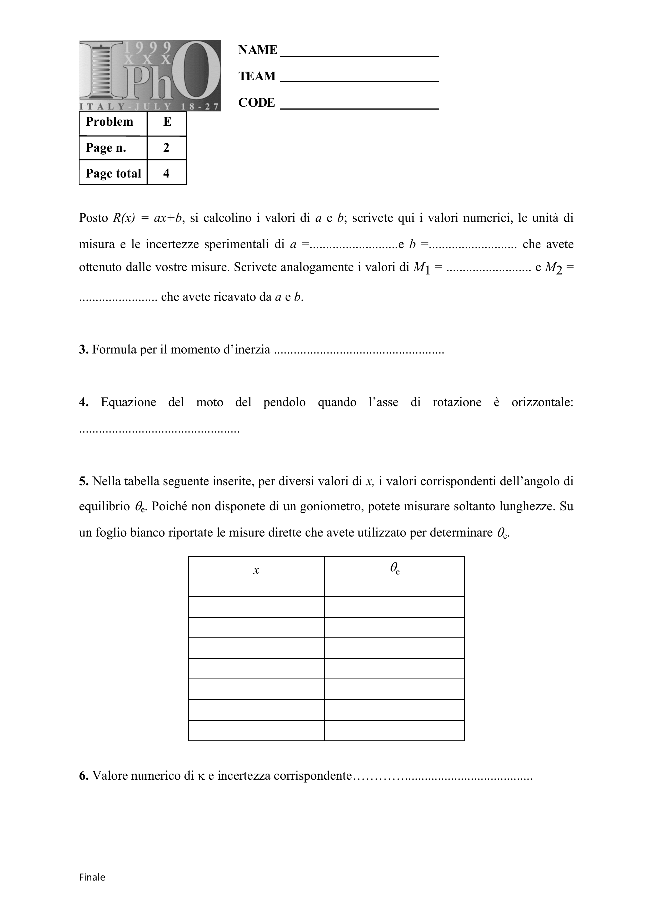
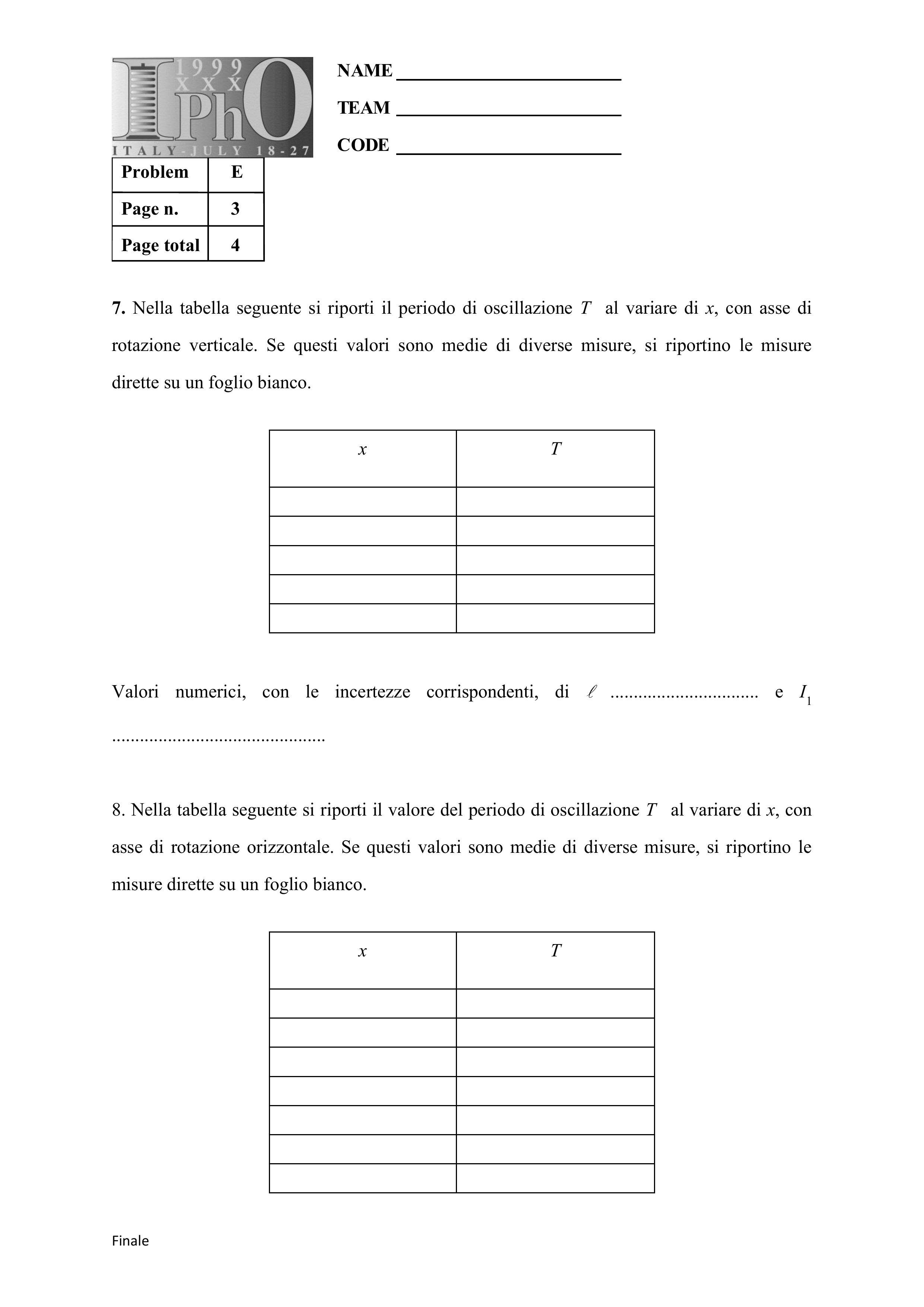
Italian answer sheets for the same experiment, numbered 1–4. The first sheet continues onto a second page.

Page n. 1

Italian answer sheet 1 with blank centre-of-mass formula, x and R(x) measurement table, and graph instruction. — Italian answer sheet 1: formulas and measurements.

Continuation of Italian answer sheet 1 with the repeated identification header and blank R(x) versus x graph grid. — Italian answer sheet 1: graph continuation.

Page n. 2

Italian answer sheet 2 with blanks for linear-fit coefficients, masses, moment of inertia, equation of motion, an equilibrium-angle table, and torsional constant with uncertainty. — Italian answer sheet 2.

Page n. 3

Italian answer sheet 3 with vertical-axis and horizontal-axis period measurement tables and blanks for rod length and outer-body moment of inertia with uncertainties. — Italian answer sheet 3.

Page n. 4

Italian answer sheet 4 with the blank T versus x graph grid and seven numbered descriptions of the period behavior. — Italian answer sheet 4.

Оригинал в Архива: exp.pdf · официални решения: exp_sol.pdf · допълнителни данни: IPhO_1999_Exp Question 1.pdf · допълнителни данни: IPhO_1999_Exp Solution l.pdf · допълнителни данни: SPESTU_I.Italian-official-derived.pdf