Съдържание
УсловиеPart A: Electric conductivity of copper, aluminum and brass (1.5 points) (1,5 т.)Part B: Thermal conductivity of copper (3.0 points) (3 т.)Part C: Estimating the heat loss and the heat capacity of copper (4.0 points) (4 т.)Part D: Thermal conductivity of brass and aluminum (1.0 points) (1 т.)Part E: The Wiedemann-Franz law (0.5 points) (0,5 т.)ОтговориРешениеIPhO 2019, Експеримент — Задача 2. Wiedemann-Franz Law
Wiedemann-Franz Law
Условие
In metals, heat is conducted primarily by electrons. For this reason, thermal and electric conductivities are related. This is known as the Wiedemann-Franz law.
In this experiment, our goal is to measure the thermal and electric properties of several metals with a reasonably high accuracy. In part A, we will measure the electric conductivity of copper, brass and aluminum. In part B, we will measure the heat conductivity of copper. In part C, we will measure the specific heat capacity of copper. In part D, we will measure the heat conductivity of brass and aluminum. Finally, in part E, we will verify the universal relation between these physical properties for the metals we studied.
In this experiment, you are not required to perform any error calculations.
Note that in part B and D there is a wait time of 15 minutes. Plan your time accordingly.
Safety instructions
Do not connect any wires or unauthorized instruments directly to the 220V/25A external power outlets. You may connect only the supplied power sources, with no modifications, to the external power outlet.
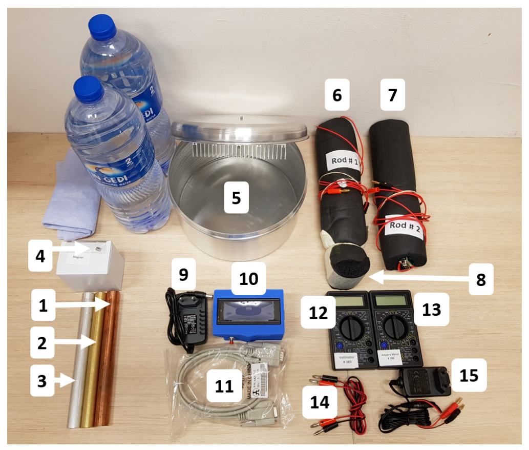
Equipment list
- Copper hollow cylindrical tube, 200.0 mm in length, with an inner hole of diameter 6.0 mm, and an outside diameter of 20.0 mm
- Brass hollow cylindrical tube, 200.0 mm in length, with an inner hole of diameter 6.0 mm, and an outside diameter of 19.0 mm
- Aluminum hollow cylindrical tube, 200.0 mm in length, with an inner hole of diameter 6.0 mm, and an outside diameter of 20.0 mm
- A small permanent magnet of mass 1.2 gram.
- Water reservoir - a specially designed pot originally intended for making a local dish called “Jachnun”, a kind of Israeli pastry. The cover of the pot includes a heat exchanger inside and a screw on top. Supplied are 4 liters of still water (2X2 liter bottles) to fill the reservoir.
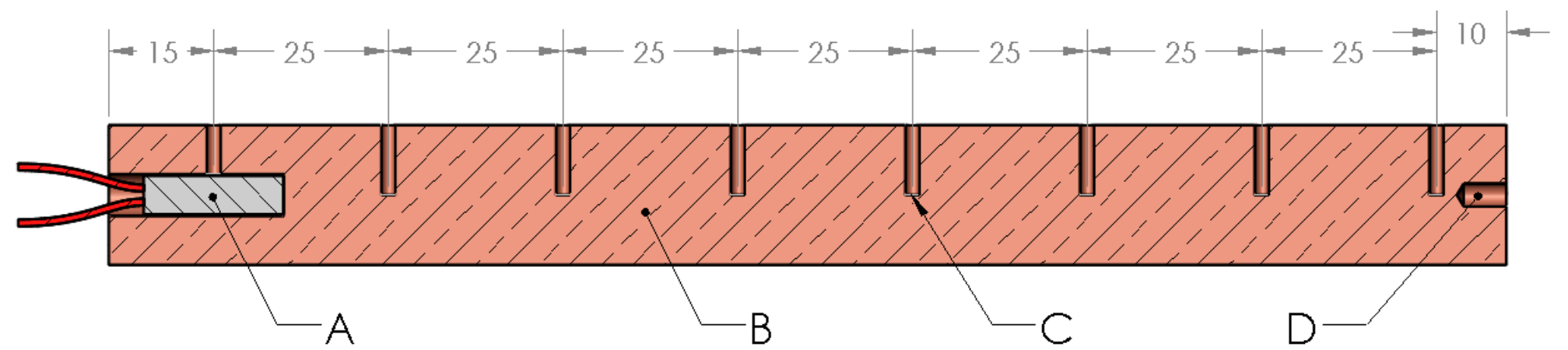
- Rod #1 - a Copper rod of diameter 20.0 mm with temperature sensors connected to the cable socket and a built-in heater connected to the red wires (figure 2.a). The red wires are intended to be connected to the DC power supply (item 15 below) through a circuit. The rod is covered with black thermally insulating foam.
- Rod #2 - Composite rod of diameter 20.0 mm, with temperature sensors connected to the cable socket and a built-in heater connected to the red wires (figure 2.b). The red wires are intended to be connected to the DC power supply (item 15 below) through a circuit. The rod is covered with black thermal insulating foam.
- Thermally insulating termination cap.
- 12V DC power supply for the digital readout box.
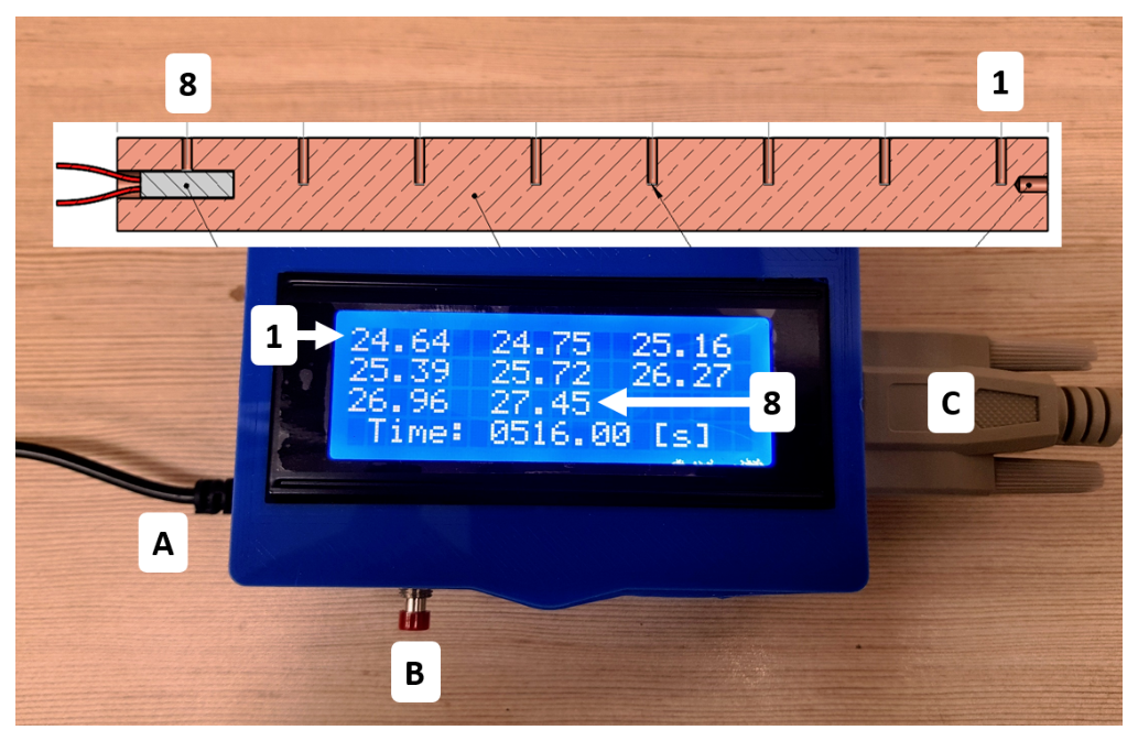
- Digital readout box. This box displays the readings of the eight thermometers and the time, see instructions below. This box is also used as a stopwatch.
- Thermometer cable that connects the rod’s thermometers to the digital readout box.
- Voltmeter - the voltmeter function selector should be set to 20 Volts DC (Figure 3).
- Ammeter - The ammeter function selector should be set to 10 Amperes DC (Figure 3).
- Electrical wires.
- 9V DC power supply for the heater connected to banana plugs.

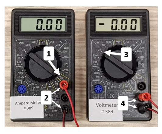
WARNINGS: 1. Only the supplied power sources (with standard AC plugs) should be connected to the external power outlet. Connecting isolated wires or other equipment to the outlet is strictly forbidden and may cause serious injury.
- Do not immerse the rods in the water.
Using the digital readout box
Connect the digital readout box to its 12V DC power supply.
The digital readout box has two operation modes, as a stopwatch and as a temperature readout. When the cable from the sensors is connected to the box, the box will switch to temperature readout mode automatically. When the sensor cable is disconnected, the box will change to stopwatch mode automatically, and the screen will show the words "Timer mode".
In temperature mode :
- Press and hold the red button for 3 seconds to reset the time
- Pressing briefly the red button will hold the reading display (while the box is still counting the time from the last reset but does not display it)
- Pressing again the red button resumes the live temperature and time display.
In stopwatch mode:
- Pressing of the red button starts the stopwatch.
- Pressing again stops the stopwatch.
- Pressing an additional time resets the stopwatch back to zero.
The readout box must be calibrated for each rod before first use. The thermometers used in the experiment are not precisely identical. Therefore, while the rod is in thermal equilibrium, we would want to calibrate to get the same reading from all sensors. To do so, first, connect one end of the thermometers cable to the rod. Then, press and hold the red button while connecting the other end of the thermometers cable to the box. Disconnecting the box from both the power or sensors cables will not erase the calibration.
WARNING: Perform calibration before connecting the rod to the reservoir, or connecting its heater to the power supply. This will guarantee that the temperature of the rod is uniform during the calibration.
If you encounter any problems with the readout box, you may find it useful to unplug the readout box from its power supply and then plug it in again. The box will remember its last calibration.
Part A: Electric conductivity of copper, aluminum and brass (1.5 points) (1,5 т.)
Theory
When a permanent magnet falls inside a hollow cylindrical conductive tube, it experiences a dissipative force due to induced eddy currents. Therefore, the magnet reaches a terminal velocity. For this geometry the terminal velocity can be expressed as:
Here is the mass of the magnet, is the electrical conductivity of the material of the tube, is the inner radius of the tube, and are the radius and the height of the magnet, respectively, is the remanent magnetization of the magnet, is the thickness of the tube wall and is a scaling function. In our case, , and . Therefore, the time it takes for the magnet to fall through the tube can be approximated by:
Here m is the length of the tube and we assume that the magnet reaches terminal velocity immediately upon its release.
The characteristics of the tube and the magnet which are needed for the calculation are:
T, m, m, kg , m, m/s
Experiment
A.1 Using the digital readout box in stopwatch mode, measure the time it takes the magnet to fall through the hollow tubes made of aluminum, copper and brass. Write down your measurements in table A1. [1 т.]
A.2 Using the equation above, find the electrical conductivities for each of the three materials. [0,5 т.]
Part B: Thermal conductivity of copper (3.0 points) (3 т.)
The goal of this section is to measure the heat conductivity of copper close to the steady state.
Theory
The thermal conductivity is defined by the equation . This equation describes a linear relation between the local temperature gradient and the local power flowing through a cross section of the material. Here, is the power flowing through a cross-section at location , is the cross-sectional area of the rod and is the temperature gradient at position .
Experiment
Connect the digital readout box to the external outlet and calibrate Rod #1. Pour 4 liters (2 bottles) of water into the pot to fully immerse the heat exchanger and close the lid.
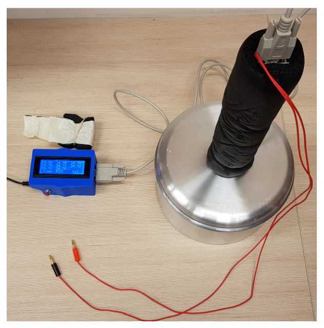
B.1 Write down the initial temperature of rod #1 when placed on the table. [0,1 т.]
Disconnect the readout cable from the rod. Remove the insulating cap and screw rod #1 onto the cover of the pot. Reconnect the cable to the readout box, as shown in figure 5. Be careful not to apply too much torque.
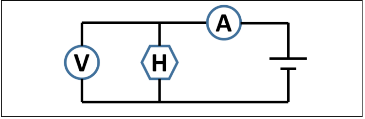
B.2 Draw a circuit that will allow you to supply power to the heater and to measure that power. Your circuit should contain the following: 9V power source, heater (already connected to the rod), the voltmeter, the ammeter and wires. You may use the wires as a switch to open and close the circuit. [0,5 т.]
The heat conductivity will be measured by applying heat power to one side of the rod while keeping the other side of the rod at the almost constant temperature of the water reservoir.
We aim to get close to a steady state for all thermometers. Connect the circuit from section B2 and apply power to the heater.
B.3 Perform appropriate measurements to compute the applied power to the heater, and write it down in the answer sheet. [0,1 т.]
Wait for 15 minutes while applying power (you can use this time to plan your experiments).
B.4 Write down in the supplied table the temperatures of all eight thermometers at approximate times: 15 min, 17.5 min, 20 min. [0,5 т.]
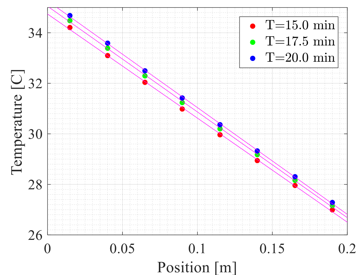
B.5 On one graph paper, draw three graphs of the temperature as a function of position for each of the measured times. These graphs will also be used in Part D. [1 т.]
B.6 Use the graph to extract the thermal conductivity of copper, , using your data from time approximately 17.5 min. Disregard any heat loss in this part. Estimate the average rate of temperature change of the rod, , at time approximately 17.5 min. [0,5 т.]
B.7 Do you expect a higher / lower / the same value of , compared to the real value of ? [0,3 т.]
Part C: Estimating the heat loss and the heat capacity of copper (4.0 points) (4 т.)
Theory
The heat capacity is defined by either of the following equations:
Here, is the net heat rate transfer to the material and is the temperature change rate. The specific heat is the heat capacity per unit mass. The mass of the copper rod should be taken as kg.
Experiment
Turn off the heater power supply. Disconnect the circuit, unscrew and place rod #1 on the table. Place the insulating termination cap onto the rod, as you found it at the beginning of the experiment. Reconnect the heater circuit and reconnect the rod to the digital readout box.
WARNING: Do not leave the heater on in this part for long periods of time without monitoring the temperature.
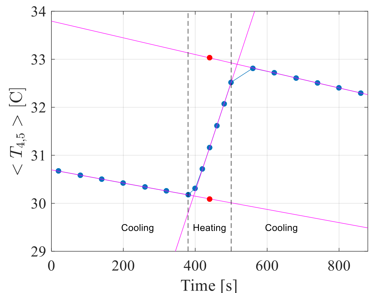
Using a sequence of cooling, heating, and cooling again, we can extract both the heat loss and the heat capacity of the material. The heating step should change the average temperature by approximately C. The necessary accuracy in this step can be achieved by a cooling-heating-cooling sequence of a total length of 10-15 minutes.
Here we aim to work near the average temperature measured close to the steady state of Part B.
In order to account for all the thermal energy stored in the rod, we would want to track its average temperature. The temperature at the center of the rod is a good approximate measure of the average temperature.
C.1 Perform a cooling-heating-cooling sequence and record your measurements in table C1, to obtain the average temperature. [1 т.]
C.2 Plot on a graph paper the average temperature versus time. [1 т.]
C.3 Using the graph, calculate the specific heat and the heat loss per unit time around the average temperature of Part B. Describe your method using diagrams and equations. [1 т.]
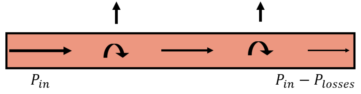
There are two main mechanisms which should be taken into account in order to improve the accuracy of the heat conductivity extracted in part B.
- There is heat loss due to radial heat transfer through the insulation.
- The system did not reach steady-state at the time of the measurement
To first order approximation, you may assume that due to these mechanisms the change per unit length of power flow along the rod, , is constant.
C.4 Write down an equation correcting to first order the thermal conductivity found in part B while taking into account both mechanisms. Use from parts B,C to express the corrected value of the thermal conductivity, and calculate its value. [1 т.]
Part D: Thermal conductivity of brass and aluminum (1.0 points) (1 т.)
Connect the insulated rod #2 to the digital readout box, and calibrate the thermometers of this rod as instructed at the beginning of Part B (while the red button is pressed, connect the insulated rod #2 to the readout box using the thermometers cable).
D.1 Write down the initial temperature of the rod when placed on the table. [0,1 т.]
Disconnect the cable and screw rod #2 onto the pot’s cover as shown in figure 4. Reconnect the cable to the readout box.
Repeat the procedure used in part B to get close to the steady state while heating.
Supply power to the heater for at least 15 minutes before making measurements.
You may assume, for the accuracy required in this part, that the rod is in steady state. In addition, you may assume that the heat loss per unit length is constant along the rod.
D.2 Write down the temperature readings from all eight thermometers of rod #2 and write down for each of its sections. [0,2 т.]
To first order approximation, you may use the same assumption as in task C.4, namely, that is constant.
D.3 Express and using your previous measurements and evaluate their numerical values. [0,7 т.]
Part E: The Wiedemann-Franz law (0.5 points) (0,5 т.)
The Wiedemann-Franz law states that, in metals where heat transport is dominated by conduction electrons, the ratio of thermal and electrical conductivities depends linearly on the absolute temperature. Moreover, the law states that the slope (known as the "Lorenz number") of this dependence is the same for most metals, and depends only on universal constants of nature. In reality, for metals at room temperature, this law holds with about accuracy.
E.1 Write down your findings for thermal and electrical conductivities ( ) in table E1. Calculate the value of for each material and display it in the same table E1, while assuming that the thermal conductivity does not depend on temperature to first order. [0,5 т.]
Отговори
Part A: Electric conductivity of copper, aluminum and brass (1.5 points), A.2 σCopper = 5.97 × 10⁷ 1/(Ω m), σAluminum = 2.98 × 10⁷ 1/(Ω m), σBrass = 1.60 × 10⁷ 1/(Ω m)
Values from the official sample measurement; each student uses their own measured times.
Part B: Thermal conductivity of copper (3.0 points), B.7 higher value
Part C: Estimating the heat loss and the heat capacity of copper (4.0 points), C.4 396 W/(m·K)
Official sample value; the solution compares it with the expected 385 W/(m·K).
Part D: Thermal conductivity of brass and aluminum (1.0 points), D.3 κBrass = 115 W/(m·K), κAluminum = 239 W/(m·K)
Official sample values.
Part E: The Wiedemann-Franz law (0.5 points), E.1 L(Copper) = 2.21 × 10⁻⁸ WΩ/K², L(Aluminum) = 2.67 × 10⁻⁸ WΩ/K², L(Brass) = 2.40 × 10⁻⁸ WΩ/K²
Official sample values.
Решение
Wiedemann-Franz Law – Solution
Part A: Electrical conductivity of metals (1.5 points) (1,5 т.)
A.1 (1.0 points)
Magnet descend time:
| Number | Copper [s] | Aluminum[s] | Brass [s] |
|---|---|---|---|
| 1 | 17.77 | 9.23 | 6.1 |
| 2 | 17.96 | 9.39 | 5.83 |
| 3 | 18.16 | 9.22 | 6.04 |
| 4 | 18.15 | 9.37 | 5.86 |
| 5 | 17.76 | 9.36 | 6.16 |
| 6 | 18.2 | 9.44 | 5.92 |
| 7 | 17.67 | 9.65 | 5.9 |
| 8 | 17.9 | 9.18 | 6.08 |
| 9 | 17.67 | 9.41 | 5.86 |
| 10 | 18.36 | 8.96 | 5.99 |
| Average | 17.96 | 9.32 | 5.97 |
A.2 (0.5 points)
| Copper | Aluminum | Brass | |
|---|---|---|---|
| Electrical conductivity |
Part B: Thermal conductivity of copper (3.0 points) (3 т.)
B.1 (0.1 points)
Rod 1 temperature : 22.76 [C]
B.2 (0.5 points)
B.3 (0.1 points)
B.4 (0.5 points)
| Time [S] | T1 [C] | T2 [C] | T3 [C] | T4[C] | T5 [C] | T6 [C] | T7 [C] | T8 [C] |
|---|---|---|---|---|---|---|---|---|
| 900 | 26.98 | 27.96 | 28.95 | 29.96 | 30.98 | 32.03 | 33.10 | 34.20 |
| 1050 | 27.16 | 28.16 | 29.17 | 30.20 | 31.240 | 32.30 | 33.38 | 34.48 |
| 1200 | 27.29 | 28.30 | 29.33 | 30.37 | 31.42 | 32.49 | 33.58 | 34.68 |
B.5 (1.0 points)
B.6 (0.5 points)
B.7 (0.3 points)
higher value
We expect a higher value of compared with the real because of 2 reasons:
- A part of the supplied heat power is lost through the side walls. Therefore, the heat transfer through the cross-section of the rod is smaller.
- Since the system is not in a steady state (), the corresponding power involved should be subtracted from the power supplied by the heater.
Part C: Heat loss and heat capacity of copper (4.0 points) (4 т.)
C.1 (1.0 points)
| 20 | 30.67 | 30.67 | 30.67 | ||||||
| 80 | 30.59 | 30.59 | 30.59 | ||||||
| 140 | 30.50 | 30.50 | 30.50 | ||||||
| 200 | 30.42 | 30.42 | 30.42 | ||||||
| 260 | 30.34 | 30.34 | 30.34 | ||||||
| 320 | 30.26 | 30.26 | 30.26 | ||||||
| 380 | 30.18 | 30.18 | 30.18 | ||||||
| 400 | 30.38 | 30.25 | 30.31 | ||||||
| 420 | 30.87 | 30.56 | 30.72 | ||||||
| 440 | 31.37 | 30.96 | 31.16 | ||||||
| 460 | 31.85 | 31.38 | 31.61 | ||||||
| 480 | 32.32 | 31.82 | 32.07 | ||||||
| 500 | 32.78 | 32.26 | 32.52 | ||||||
| 560 | 32.88 | 32.75 | 32.81 | ||||||
| 620 | 32.73 | 32.70 | 32.72 | ||||||
| 680 | 32.61 | 32.61 | 32.61 | ||||||
| 740 | 32.51 | 32.51 | 32.51 | ||||||
| 800 | 32.40 | 32.40 | 32.40 | ||||||
| 860 | 32.30 | 32.30 | 32.30 |
C.2 (1.0 points)
C.3 (1.0 points)
The purpose of this part is to correct to first order the result in part B. Hence, every solution within accuracy is accepted (see marking scheme).
Solution 1 (using slopes):
Where is the average of both cooling slopes.
Which is off the correct value.
Solution 2 (using jump):
Where is the average of the two cooling slopes, and is the extrapolated jump in temperature half way though the heating time interval.
which is the correct value.
C.4 (1.0 points)
The temperature gradient is proportional to the local heat flow.
To first order, the average temperature gradient will be proportional to the average heat flow. Therefore, the temperature gradient will be proportional to :
Which gives an error of error compared to expected . We expect a systematic error (see appendix).
Part D: Thermal conductivity of multiple metals (1.0 points) (1 т.)
D.1 (0.1 points)
D.2 (0.2 points)
Time of measurement:
| 41.68 | 40.51 | 38.51 | 34.65 | 32.47 | 30.71 | 29.63 | 28.62 |
D.3 (0.7 points)

Part E: The Wiedemann-Franz law (0.5 points) (0,5 т.)
E.1 (0.5 points)
| Copper | Aluminum | Brass | |
|---|---|---|---|
| Electric conductivity | |||
| Heat conductivity | 396 | 239 | 115 |
| Lorenz coefficient |
Оригинал в Архива: exp2.pdf · официални решения: exp2_sol.pdf