Съдържание

IZhO 2015, Експеримент — Задача 1. Resistance of graphite

Оригинал на условието (PDF)Съобщи за грешка

Всички материали от IZhO 2015

XI International Zhautykov Olimpiad/Experimental Competition — EXPERIMENTAL COMPETITION, 14 January, 2015 · 14 януари 2015 г. · 15 т.

Please read the instructions first:

The Experimental competition consists of one problem. This part of the competition lasts 3 hours.
Please only use the pen that is provided to you.
You can use your own non-programmable calculator for numerical calculations. If you don’t have one, please ask for it from Olympiad organizers.
You are provided with Writing sheet and additional papers. You can use the additional paper for drafts of your solutions but these papers will not be checked. Your final solutions which will be evaluated should be on the Writing sheets. Please use as little text as possible. You should mostly use equations, numbers, figures and plots.
Use only the front side of Writing sheets. Write only inside the bordered area.
Fill the boxes at the top of each sheet of paper with your country (Country), your student code (Student Code), the question number (Question Number), the progressive number of each sheet (Page Number), and the total number of Writing sheets (Total Number of Pages). If you use some blank Writing sheets for notes that you do not wish to be evaluated, put a large X across the entire sheet and do not include it in your numbering.
At the end of the exam, arrange all sheets for each problem in the following order:
- Used Writing sheets in order;
- The sheets you do not wish to be evaluated
- Unused sheets and the printed question.
Place the papers inside the envelope and leave everything on your desk. You are not allowed to take any paper or equipment out of the room

Условие

Instruments and equipment: graphite rod, multimeter, power source (battery 4.5 V), fixed resistors 1.0 Ohm and 10 Ohm, variable resistor (use the sharp edge of the plastic ruler for its adjustment), connecting wires, stopwatch, vessel with snow.

Warning! Be careful, since the graphite rod is very fragile and may be easily broken. Connect it to a circuit with the clips called the "crocodile".

Graphite electrical resistance $R_g$ depends on its temperature. One can approximate that this dependence is linear

R_g = R_0(1 + \alpha\Delta T),

wherein $\Delta T$ denotes the temperature difference between the room and the rod, $R_0$ is the resistance of the graphite rod at room temperature, $\alpha$ stands for the temperature coefficient of graphite resistance.

The room temperature will be announced during the experimental competition.

It can also be assumed that the power of the heat dissipated into the ambient air is proportional to the temperature difference between the rod and the air

P = \beta\Delta T,

where $\beta$ is the heat transfer coefficient.

Part 1. The current-voltage characteristic of a graphite rod

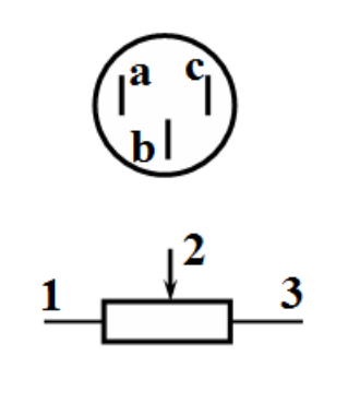
Top view of the variable resistor as a circle with three pins labelled a, c (top) and b (bottom); below it the circuit symbol of a variable resistor: a rectangle between terminals 1 and 3 with a sliding contact arrow labelled 2.

1.1 Use the multimeter (in this paragraph, use it in the mode of resistance measurements) to determine which of its pins corresponds to the sliding lead (indicated in the figure by 2). [0,2 т.]

1.2 Measure the dependence of the current through the graphite rod, which is placed in the air, on the voltage across it.

For the measurements, use the multimeter in the mode of voltmeter since it works very unstable in the mode of ammeter. To measure current, use the resistor of 1.0 ohms. To change the current in a circuit use the variable resistor. Bear in mind that when the current flows through the rod it takes some time for the temperature to change. After changing the value of the variable resistor by turning its knob, you should wait at least 30-40 seconds before taking the readings.

1.2.1 Draw schematically an electrical circuit that you used for taking measurements. [0,5 т.]

1.2.2 Plot the graph of the dependence obtained. Derive a theoretical formula that describes this dependence. [3 т.]

1.2.3 Calculate the electric resistivity of graphite at room temperature. Estimate its experimental error. The relative error of each resistor is 5%. The rod diameter is $d = 1.0 \pm 0.05\ \mathrm{mm}$ . To measure the length the graph paper may be used. [1,1 т.]

1.2.4 Show theoretically that in the steady state the electrical resistance of the graphite rod depends linearly on the power $P$ released in it due to the current flow

R_g = R_0(1 + \gamma P). \qquad (1)

[0,2 т.]

1.2.5 Using the obtained experimental data, calculate the dependence of the resistance of the graphite rod on the power $R_g(P)$ . Plot the corresponding graph. [0,7 т.]

1.2.6 Using the corresponding graph write down a range of powers for which formula (1) holds. Evaluate the value of $\gamma$ for this particular range. Error estimation is not required. [0,5 т.]

1.3 Measure the dependence of the current through the graphite rod on the voltage across it $I(U)$ , when the rod is immersed into the melting snow.

1.3.1 Plot the graph of the obtained dependence. [2,6 т.]

1.3.2 Evaluate the temperature coefficient of graphite resistance and estimate its experimental error $\Delta\alpha$ . [1,2 т.]

Part 2. Cooling of the graphite rod

To measure small changes in resistance it is preferable to use a bridge circuit (see. Fig.). One of the wires connected to the battery can be placed in two positions:

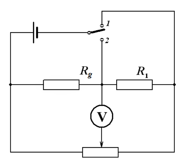
Bridge circuit: a battery connected through a switch with positions 1 and 2; the graphite rod R_g and resistor R_1 in series on the upper branch, a voltmeter V between their junction and the sliding contact of the variable resistor on the lower branch.

1 – measurement mode;

2 – heating mode.

By turning the knob of the variable resistor, it can be ensured that the voltage across the voltmeter is equal to zero (or close to it). In this case the bridge is called balanced. Take resistor of 10 ohms as a resistor $R_1$ .

If you change the resistance $R_g$ of the graphite rod, the voltage across the voltmeter turns non zero. In this case it can be shown independently (you do not need to do that), that the voltage across the voltmeter is proportional to the change in the resistance of the graphite rod.

2.1 Without heating the rod, place the battery wire in the measurement mode (position 1). Use the knob of the variable resistor to make the multimeter readings close to zero (as close as possible).

Quickly switch the same battery wire in position 2, heat the rod by waiting for at least 1 minute. Then quickly switch the battery wire back in position 1 and measure the dependence of voltage on time. [3 т.]

2.2 Plot the dependence obtained. [0,4 т.]

2.3 If the rod is connected to a DC voltage source, but its temperature differs from the stationary one $\bar{T}$ ,, then the change of temperature $T$ over time $t$ is approximately governed by the equation

\frac{dT}{dt} = -\frac{1}{\tau}(T - \bar{T}).

Using the experimental data verify the validity of this equation. Calculate the value of the characteristic time $\tau$ of thermal equilibration. Error estimation is not required. [1,6 т.]

Отговори

Решение

Part 1. The current-voltage characteristic of a graphite rod

1.1 Using the ohmmeter it is easy determine that the the sliding lead is b.

1.2.1 To measure the current-voltage characteristics of the graphite rod, the traditional circuit, shown in the figure, can be used. When the voltmeter is thrown into position 1 the voltage across the graphite rod is measured, whereas in position 2 the measured voltage is the one across the resistor $R_0 = 1{,}0\ \mathrm{Ohm}$ . If the voltage is measured in volts, then the voltage across the resistor is numerically equal to the current strength in the circuit in amps.

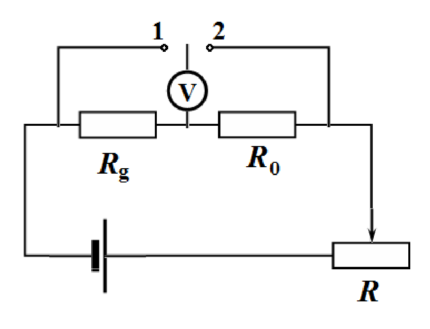
Circuit for measuring the current-voltage characteristic: graphite rod R_g and resistor R_0 in series with a battery and a variable resistor R (sliding contact arrow); a voltmeter V connected at the junction of R_g and R_0 with a switch whose other end goes to position 1 (across R_g) or position 2 (across R_0).

It is possible to connect the variable resistor as a potentiometer, although in this case the maximum current in the circuit will be slightly less.

1.2.2 The results of measurements of the current-voltage characteristic of the graphite rod are presented in Table 1. This table also shows the power values calculated via

P = UI \qquad (1)

as well as the resistance of the graphite rod

R = \frac{U}{I}. \qquad (2)

Table 1. Measurements made in the air

U, V	I, A	P, W	R, Ohm
0,150	0,040	0,0060	3,750
0,188	0,050	0,0094	3,760
0,202	0,054	0,0109	3,741
0,261	0,070	0,0183	3,729
0,304	0,081	0,0246	3,753
0,411	0,109	0,0448	3,771
0,470	0,124	0,0583	3,790
0,742	0,199	0,1477	3,729
0,907	0,243	0,2204	3,733
1,155	0,312	0,3604	3,702
1,486	0,406	0,6033	3,660
1,570	0,430	0,6751	3,651
2,280	0,640	1,4592	3,563

1.2.3 The current-voltage characteristic of the graphite rod is shown in the figure below.

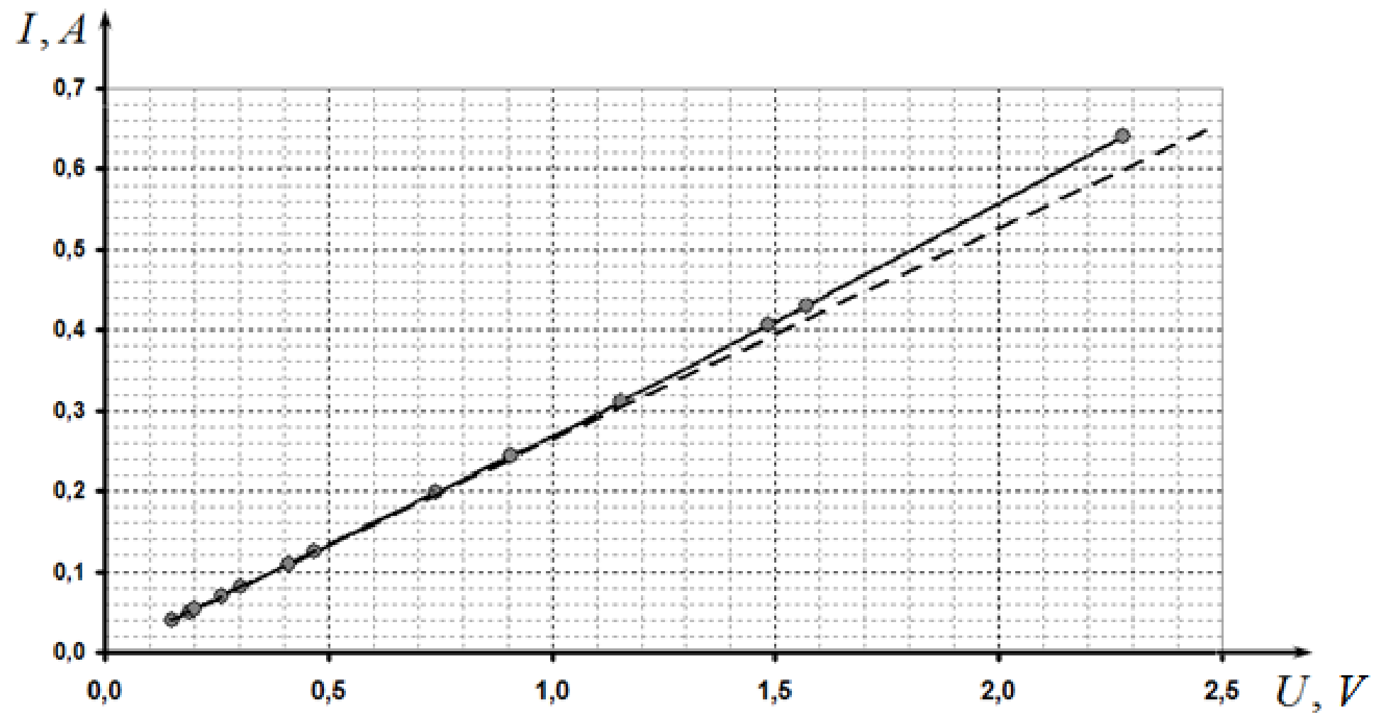
Graph of current I, A (0 to 0.7) against voltage U, V (0 to 2.5) for the rod in air: measured points on a solid line that bends slightly upward above a dashed straight line at higher voltages.

It can be seen that the curve deviates somewhat up from the linear proportionality which is prescribed to decrease in the resistance of the graphite when the temperature increases.

Derivation of the theoretical formula.

In the steady state the condition of thermal equilibrium is written as:

\frac{U^2}{R_0(1 + \alpha\Delta T)} = \beta\Delta T. \qquad (3)

Solving the quadratic equation for the temperature difference gives rise to

\begin{gathered} \frac{U^2}{R_0} = \beta\Delta T(1 + \alpha\Delta T) \;\Rightarrow\; \alpha\beta(\Delta T)^2 + \beta\Delta T - \frac{U^2}{R_0} = 0 \\ \Delta T = \frac{-\beta \pm \sqrt{\beta^2 + 4\frac{U^2}{R_0}\alpha\beta}}{2\alpha\beta} \end{gathered}. \qquad (4)

From the data obtained it follows that the temperature coefficient of graphite resistance is negative. In addition, it can be shown that from the two roots of equation (3) the smaller one should be chosen (with + sign), since it corresponds to a stable thermal equilibrium. Therefore, the theoretical dependence has the form

I = \frac{U}{R_0(1 + \alpha\Delta T)} = \frac{U}{R_0\left(1 + \frac{-\beta + \sqrt{\beta^2 + 4\frac{U^2}{R_0}\alpha\beta}}{2\beta}\right)} \approx \frac{U}{R_0\left(1 + \frac{U^2}{R_0}\frac{\alpha}{\beta}\right)} \approx \frac{U}{R_0}\left(1 - \frac{U^2}{R_0}\frac{\alpha}{\beta}\right). \qquad (5)

The last two expressions are approximations valid for small $\alpha$ .

1.2.3 For a more accurate calculation of the resistance of the graphite rod at room temperature, only several data points at low voltages (less than 0.5V) should be taken at which the rod remains practically unheated. Then, the method of least squares must be employed to evaluate the slope, which is equal to the rod resistance.

Calculation of the obtained experimental data leads to the following result

R_0 = (3{,}78 \pm 0{,}03)\,\mathrm{Ohm}.

To calculate the resistivity of use is the following formula

R = \rho\frac{4l}{\pi d^2} \;\Rightarrow\; \rho = \frac{\pi d^2}{4l}R = \frac{\pi\cdot(1{,}0\cdot 10^{-3})^2}{4\cdot 5{,}0\cdot 10^{-2}}3{,}78 = 5{,}93\cdot 10^{-5}\,\mathrm{Onm}\cdot\mathrm{m}

Here $l = (5{,}0 \pm 0{,}2)\,\mathrm{sm}$ is the length of the rod between the leads.

The calculation of experimental error is given by the formula

\Delta\rho = \rho\sqrt{\left(\frac{\Delta R}{R}\right)^2 + \left(2\frac{\Delta d}{d}\right)^2 + \left(\frac{\Delta l}{l}\right)^2} = 5{,}93\cdot 10^{-5}\sqrt{\left(\frac{0{,}03}{3{,}78}\right)^2 + \left(2\frac{0{,}05}{1}\right)^2 + \left(\frac{0{,}2}{5}\right)^2} = 6\cdot 10^{-6}\,\mathrm{Ohm}\cdot\mathrm{m}

The final result is written as

\rho = (5{,}9 \pm 0{,}6)\cdot 10^{-5}\,\mathrm{Ohm}\cdot\mathrm{m} \qquad (6)

1.2.4 In the steady state the power, released when the current flows, is equal to the power of the heat losses:

P = \beta\Delta T \;\Rightarrow\; \Delta T = \frac{P}{\beta},

Therefore, the dependence of the resistance on the power takes the form

R_g = R_0(1 + \alpha\Delta T) = R_0(1 + \frac{\alpha}{\beta}P)). \qquad (7)

1.2.5 The dependence of the resistance on the dissipated power is shown in the figure.

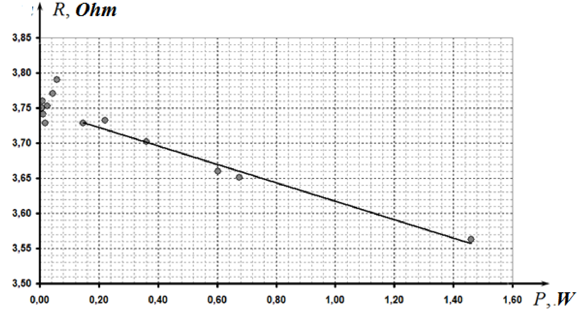
Graph of resistance R, Ohm (3.50 to 3.85) against power P, W (0 to 1.60): scattered points near P = 0 around 3.73–3.79 Ohm, and a straight decreasing line from about (0.15; 3.73) to (1.46; 3.56) through the higher-power points.

1.2.6 The linearity of this dependence is observed at powers larger than $0{,}2\,\mathrm{W}$ .

The coefficients of this dependence $R = aP + b$ , calculated using the least square method, are found as $a = 0{,}13\frac{\mathrm{Ohm}}{\mathrm{W}}$ , $b = 3{,}75\,\mathrm{Ohm}$ , consequently, the coefficient in formula (3) is evaluated as $\gamma = \frac{a}{b} = 0{,}035\,\mathrm{W}^{-1}$ .

1.3.1 The results of measurements of the current-voltage characteristic of the rod, placed in the snow, are given in Table 2 and the corresponding graph is shown in the figure below.

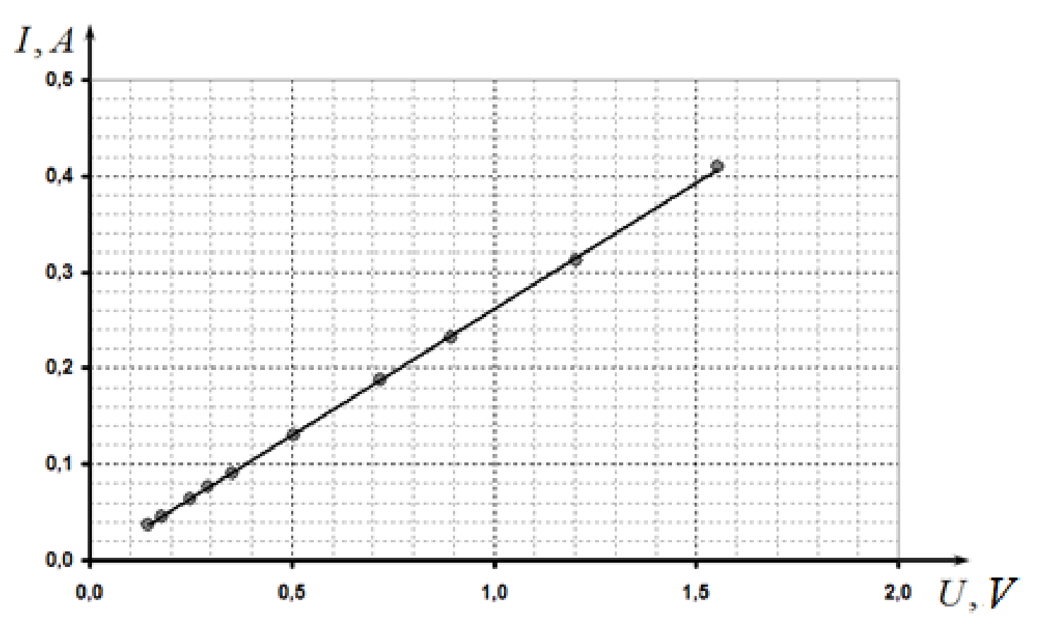
Graph of current I, A (0 to 0.5) against voltage U, V (0 to 2.0) for the rod in snow: ten measured points on an almost straight line from (0.14; 0.04) to (1.55; 0.41).

Table 2

U, V	I, A
0,144	0,037
0,177	0,045
0,248	0,064
0,292	0,076
0,354	0,091
0,504	0,130
0,721	0,188
0,895	0,232
1,205	0,312
1,554	0,409

In this case there is also a weak nonlinearity with increasing power. Therefore, to calculate the resistance at zero temperature and only several initial points at low resistance should be used. Calculation for the first five points leads to the following value

R_g = (3{,}88 \pm 0{,}03)\,\mathrm{Ohm}.

Since this value should obey the formula $R_g = R_0(1 + \alpha\Delta T)$ , the temperature coefficient of the resistance can be calculated as

\alpha = \frac{1}{\Delta T}\left(\frac{R_g}{R_0} - 1)\right) = -\frac{1}{20^{\circ}}\left(\frac{3{,}88}{3{,}78} - 1\right) = -1{,}3\cdot 10^{-3}\,\mathrm{K}^{-1}.

The experimental error is mainly determined by the measurement error of resistance, thus it can be evaluated via the formula

\Delta\alpha = \sqrt{\left(\frac{\Delta R_g}{\Delta T\cdot R_0}\right)^2 + \left(\frac{R_g\Delta R_0}{\Delta T\cdot R_0^2}\right)^2} \approx 6\cdot 10^{-4}\,\mathrm{K}^{-1}..

Part 2. Cooling of the graphite rod

2.1 The results of measurements of time time needed to achieve the specified voltage are shown in Table 3 and the corresponding graph is shown n the figure below.

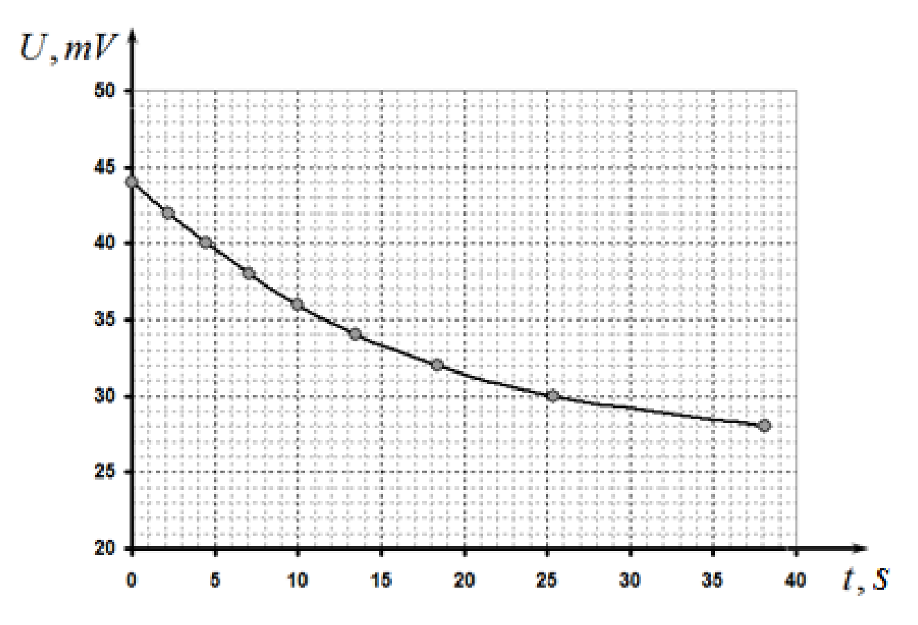
Graph of bridge voltage U, mV (20 to 50) against time t, s (0 to 40): points on a decreasing convex curve from 44 mV at t = 0 to 28 mV at about 38 s.

Table 3

U, mV	t, s	$\ln(U - \bar{U})$
44	0,00	3,045
42	2,22	2,944
40	4,45	2,833
38	7,03	2,708
36	9,99	2,565
34	13,50	2,398
32	18,42	2,197
30	25,38	1,946
28	38,14	1,609

Since the voltage is proportional to the measured voltage change and the resistance change is proportional to the change in temperature, the dependence measured coincides, up to an unimportant factor, with the temperature dependence on time.

The solution ot the equation

\frac{\Delta T}{\Delta t} = -\frac{1}{\tau}(T - \bar{T})

is the exponential function

(T - \bar{T}) = (T - \bar{T})_0\exp\left(-\frac{t}{\tau}\right). \qquad (8)

To determine the characteristic cooling time, the resulting dependence should be drawn in a semilogarithmic scale, $\ln(U - \bar{U})$ against the time. For numerical calculations it is necessary to measure the steady-state voltage value (achieved after waiting for a few minutes). In our measurements. Table 3 shows the results of calculations of logarithms.

The following figure shows the graph on the semilogarithmic scale.

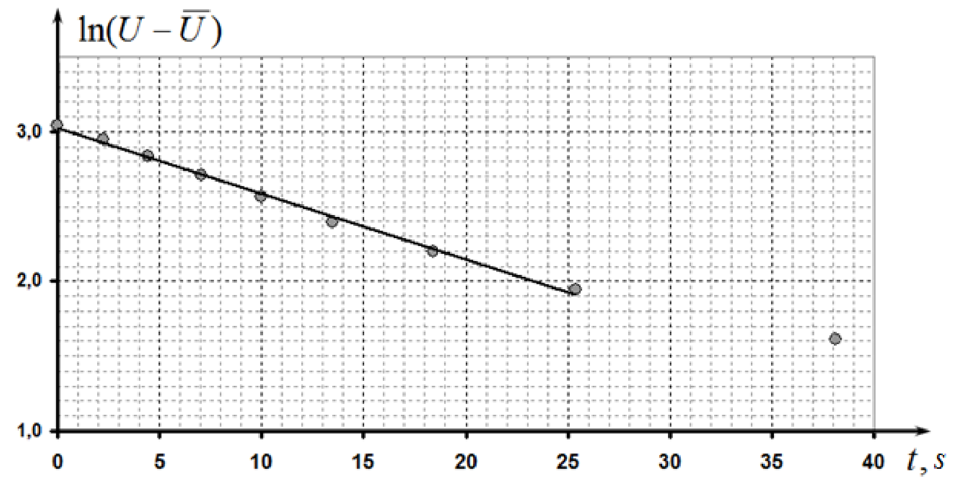
Semilogarithmic graph of ln(U − Ū) (1.0 to about 3.5) against t, s (0 to 40): points lie on a straight decreasing line from about 3.05 at t = 0 to 1.95 at t = 25 s; the last point (38 s; 1.61) lies below the line.

The slope coefficient of the obtained almost linear dependence is found as $a = -0{,}044\,\mathrm{s}^{-1}$

Consequently, the characteristic time of thermal equilibration is equal to $\tau = -\frac{1}{a} \approx 23\,\mathrm{s}$ .

Marking scheme

№	Content	points
1.1	Sliding lead is b	0,2
1.2.1	Circuit:	0,5
	- the resistor and the graphite rod are connected in series;	0,2
	- voltages are measured on the resistor and the graphite rod;	0,1
	- ability to vary the net electric current (the variable resistor connected in series, or as a voltage divider);	0,1
	- the source is correctly connected;	0,1
1.2.2	marked only if the deviation from the table in the solution is less than 50%	3,0
	Measurements :
	- 10 points or more (7-9 points; 5-6 points; less than 5 points)	1,5(0,8; 0,5;0)
	- minimum voltage less than 0,2 V;	0,2
	- maximum voltage larger than 2 V;	0,2
	- deviation to the top from the linear dependence;	0,3
	Graph:
	- axes are named and ticked;	0,1
	- points in the Table correspond to the points in the graph;	0,2
	- smooth line is drawn;	0,1
	Theoretical formula (thermal equilibrium equation, quadratic equation for temperature, smaller root is chosen, substitution into Ohm’s law)	0,4
1.2.3	The resistance of the rod is calculated:	1,1
	- voltages not larger than 0,3 V are only used;	0,2
	- all points in the stated range are used for calculation (not less than 5);	0,2
	(by 2points, by 1 point)	(0,1; 0,05)
	- the calculated value of the resistance is in the range 3,5-4,5 Ohm (3,0 – 5,0 Ohm);	0,1 (0,05)
	the length of the rod is measured (not larger than 5 sm);	0,1
	Fromula for $\rho$ ;	0,1
	$\rho$ is calculated: in the range ±20% (±50%);	0,3 (0,1)
	Error is estimated (any method)	0,1
1.2.4		0,2
	Equation for thermal equilibrium;	0,1
	Formula for $R(\Delta T)$	0,1
1.2.5		0,7
	Formula for the power;	0,05
	Formula for the resistance;	0,05
	Calculations for all points;	0,2
	Graph:
	- axes are named and ticked;	0,1
	- points in the Table correspond to the points in the graph;	0,2
	- smooth line is drawn;	0,1
1.2.6		0,5
	The linear range is stated with the power larger than 0,2 W	0,1
	The slope is calculated by all points (by 2 points)	0,2 (0,1)
	Formula for calculation;
	-numerical value is in the range 0,025-0,045 W $^{-1}$ (0,01 – 0,06)	0,2 (0,1)
1.3.1	marked only if the deviation from the table in the solution is less than 50%	2,6
	Measurements :
	- 10 points or more (7-9 points; 5-6 points; less than 5 points)	1,5 (0,8; 0,5)
	- minimum voltage is less than 0,2 V;	0,2
	- maximum voltage is larger than 1,5 V;	0,2
	- almost linear dependence is obtained;	0,1
	- small deviation from the linear dependence to the top	0,2
	Graph:
	- axes are named and ticked;	0,1
	- points in the Table correspond to the points in the graph;	0,2
	- smooth line is drawn;	0,1
1.3.2	The resistance is calculated for the snow temperature:	1,2
	- points with voltage less than 0,5 V are only used;	0,2
	- calculation by all points (by 2 points, by 1 point);	0,2 (0,1, 0,05)
	- the numerical value is in the range 3,5-4,5 Ohm (3,0 – 5,0 Ohm);
	- the resistance is larger than at room temperature;	0,1 (0,05)
	- formula for the temperature coefficient of resistance;	0,1
	- negative value;	0,1
	- numerical value is in the range ±50% (±75%);	0,1
	- error is estimated;	0,2(0,1)
	- error is larger than 50%	0,1
		0,1
2.1		3
	marked only if the deviation from the table in the solution is less than 50%
	Measurement:
	- not less than 7 points (5-6 points; less than 5 points)	2 (1,5; 1)
	- decreasing dependence with convexity directed downward;	0,3
	The range of voltages is 1,5 larger;	0,3
	- there is a limiting value of the voltage;	0,4
2.2	Graph:	0,4
	- axes are named and ticked;	0,1
	- points in the Table correspond to the points in the graph;	0,2
	- smooth line is drawn;	0,1
2.3	Evaluation of the time equilibration:	1,6
	- by graph (the slope to the steady value);	0,5
	- by 1-2 points;	0,2
	- semilogarithmic linearization is applied;	1,0
	- numerical value is in the range 20-30s (15-40S, 10-45s)	0,6 (0,4; 0,2)

Оригинал в Архива: IZhO-2015-Exp_eng.pdf · официални решения: IZhO-2015-Exp_eng_sol.pdf