Съдържание

Условие Why are there more oncoming cars than overtaking cars?Elastic collision The simplest Fermi acceleration model Отговори Решение

IZhO 2023, Теория — Задача 2. Fermi acceleration

Оригинал на условието (PDF)Съобщи за грешка

Всички материали от IZhO 2023

XIX International Zhautykov Olympiad/Theoretical Competition · 2 февруари 2023 г. · 10 т.

Please read this first:

THEORETICAL COMPETITION

February 2, 2023

The duration of the theoretical competition is 4 hours. There are three problems.
You can use your own calculator for numerical calculations.
You are provided with Writing sheet and additional white sheets of paper. You can use the additional sheets of paper for drafts of your solutions, but these sheets will not be graded. Your final solutions should be written on the Writing sheets. Please use as little text as possible. You should mostly use equations, numbers, figures, and plots.
Use only the front side of Writing sheets**.** Write only inside the boxed areas.
Start putting down your solution to each problem on a new Writing sheet.
Fill in the boxes at the top of each Writing sheet with your country (Country), your student code (Student Code), problem number (Question Number), the progressive number of each Writing sheet (Page Number), and the total number of Writing sheets used (Total Number of Pages). If you use some blank Writing sheets for notes that you do not wish to be graded, put a large X across the entire sheet and do not include it in your numbering.

SOLUTIONS TO THE PROBLEMS OF THE THEORETICAL COMPETITION

Attention. Points in grading are not divided!

Условие

Cosmic rays contain extremely high energy particles. A possible mechanism for the appearance of such particles is called Fermi acceleration.

Fermi acceleration is a stochastical mechanism for the acceleration that charged particles experience when they are repeatedly reflected, usually by magnetic mirrors. In this problem, we consider the main ideas underlying this paradoxical, at first glance, phenomenon.

Why are there more oncoming cars than overtaking cars?

On a motorway with three lanes A, B, C, cars move at a constant speed in one direction: along the central lane B, a car moves at a speed of $v = 90\ \mathrm{km/h}$ ; cars move along lane A at speeds $v - \Delta v = 80\ \mathrm{km/h}$ ; cars move along lane C at speeds $v + \Delta v == 100\ \mathrm{km/h}$ . The distance between cars is the same on each of lanes A and C, the number of cars per unit of lane length for each of them is $n = 5.0\ \mathrm{km^{-1}}$ .

Consider the car moving in lane B.

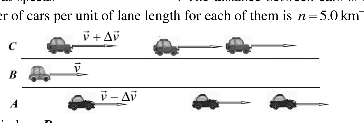
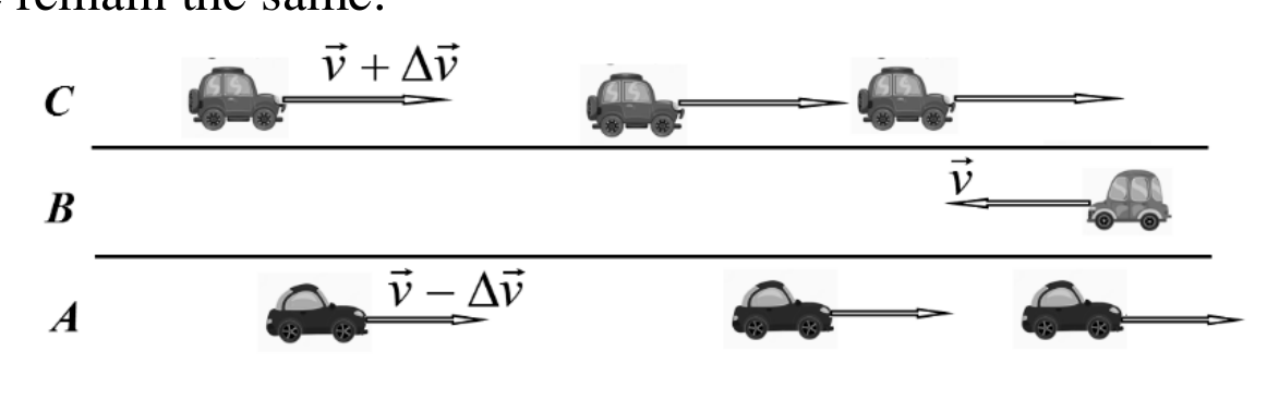
Three lanes drawn from top to bottom as C, B, A separated by two horizontal lines; in lane C three cars move to the right with velocity arrows labelled v + Δv; in lane B one car moves to the right with arrow v; in lane A three cars move to the right with arrows labelled v − Δv.

The same three lanes C, B, A: in lanes C and A three cars each move to the right with arrows v + Δv and v − Δv; in lane B a single car at the right moves to the left with the arrow v pointing left.

2.1 Calculate how many cars $N_1$ in lane A overtake the car B within the time period of $t = 1.0\ \mathrm{min}$ , as well as the time $\tau_1$ between two consecutive overtakes.

2.2 Calculate how many cars $N_2$ in lane C overtake the car in lane B within the time period of $t = 1.0\ \mathrm{min}$ , as well as the time $\tau_2$ between two consecutive overtakes.

Now let the car move in lane B towards the cars moving in lanes A and C. The speeds of all cars and their density on each lane remain the same.

2.3 Calculate the number of cars $N_3$ in lane A and $N_4$ in lane C that the car B encounters within the time period of $t = 1.0\ \mathrm{min}$ , as well as the corresponding times $\tau_3$ and $\tau_4$ between two consecutive encounters.

Elastic collision

In this part, we consider the classical problem of elastic collision of two bodies. The main purpose of this consideration is to determine the conditions under which the kinetic energy of one of the selected bodies increases as a result of the collision.

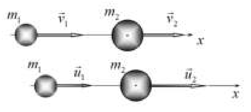
Two elastic balls, whose masses are equal to $m_1$ and $m_2$ , respectively, move along the axis $x$ . The speed of the first ball before the collision is $v_1$ , whereas the speed of the second is $v_2$ . Let us denote the speeds of the balls after an absolutely elastic central collision as $u_1$ and $u_2$ , respectively. The speeds of the balls should be understood as the projections of their velocities on the $x$ axis, therefore, they can be both positive and/or negative.

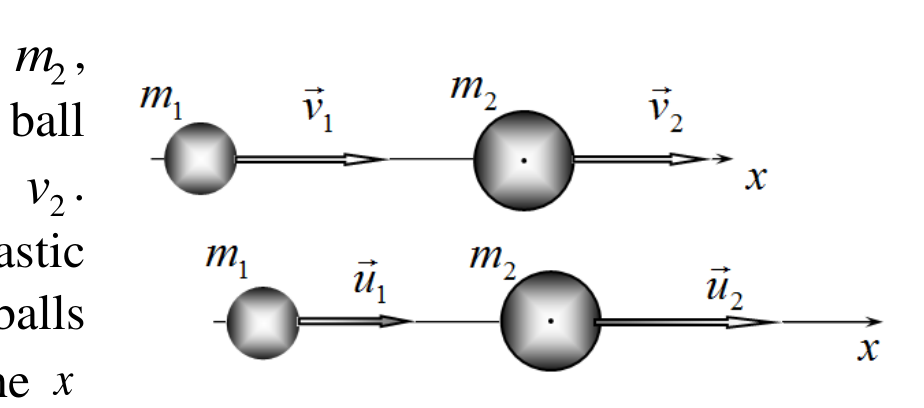
Two rows along an x axis: in the upper row a small ball m1 with velocity arrow v1 and a larger ball m2 with velocity arrow v2, both pointing right; in the lower row the same balls m1 and m2 with velocity arrows u1 and u2 pointing right.

2.4 Express the velocities of the balls $u_1$ and $u_2$ after the collision in terms of their velocities before the collision $v_1$ and $v_2$ , as well as their masses.

Let us denote the ratio of the ball masses as $\mu = \frac{m_2}{m_1}$ , the ratio of the speeds of the first ball after and before the collision as $\eta_1 = \frac{u_1}{v_1}$ and the ratio of the velocities of the balls before the collision as $\eta_2 = \frac{v_2}{v_1}$ . For definiteness, consider that $v_1 > 0$ .

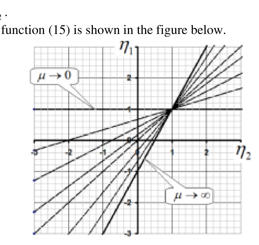
2.5 Draw a set of graphs that represents the dependence of the parameter $\eta_1$ on the parameter $\eta_2$ for all characteristic values of the ball mass ratios $\mu$ .

2.6 Find the relation between the parameters $\eta_2$ and $\mu$ , at which the first ball increases its energy as a result of the collision.

2.7 Consider the case of a light ball colliding with a heavy one such that $m_2 \gg m_1$ . In this limiting case, find the speed of the first ball $\tilde{u}_1$ after the collision and determine the range of velocities $\eta_2$ of the heavy ball before the collision, at which the energy of the light ball increases as a result of the collision.

The simplest Fermi acceleration model

A massive plate, located perpendicular to the $x$ axis, performs harmonic oscillations in the direction of the $x$ axis. The oscillation amplitude is $A$ with the period being $T$ . Light balls move with equal speeds $u$ in the direction of the plate along the $x$ axis such that the times of ball arrivals to the still plate are randomly and uniformly distributed.

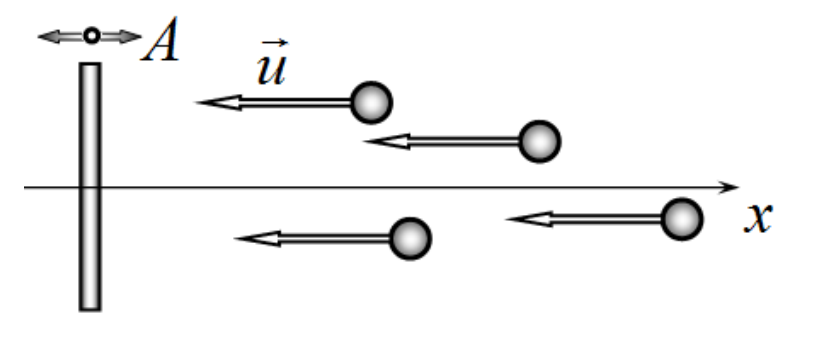
A vertical plate crossing the horizontal x axis, with a small double arrow above it marked A (the oscillation amplitude); to the right four balls on arrows labelled u move to the left, towards the plate.

Graph of x versus t with levels A and −A and times T and 2T marked: a dotted cosine curve starting at A, and a solid piecewise-linear zigzag between A and −A with the same period approximating it.

2.8 Express the maximum speed of the plate $V_0$ in terms of the amplitude and period of its oscillations.

2.9 Calculate the fraction $\varphi$ of incident balls that are to increase their kinetic energy after the collision. Express your answer in terms of $u$ and $V_0$ . For a numerical estimate, consider the following two cases separately: a) $u = 1.5V_0$ ; b) $u = 0.50V_0$ .

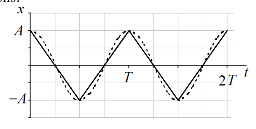
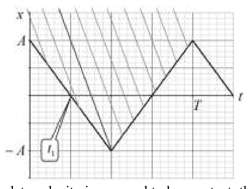
Let us approximate the harmonic law of the plate motion by a piecewise linear function, see the figure below, i.e. assume that the modulus of the plate speed remains constant at the same values of the amplitude and period of oscillations.

2.10 Express the value of the plate speed modulus $V$ in terms of the amplitude and period of its oscillations.

2.11 Calculate how many times $\varepsilon = \frac{E}{E_0}$ the average energy of the incident balls changes, where $E_0$ is the kinetic energy of the balls before the collision, and $E$ symbolizes the average energy of the balls after the collision with the oscillating plate. For a numerical estimate, consider the following two cases separately: a) $u = 1.5V$ ; b) $u = 0.50V$ .

Отговори

Why are there more oncoming cars than overtaking cars?, 2.1 $N_1 = n\Delta v t \approx 0.83,\quad \tau_1 = \frac{1}{n\Delta v} = 0.02\ \mathrm{h} = 72\ \mathrm{s}$
Why are there more oncoming cars than overtaking cars?, 2.2 $N_2 = n\Delta v t \approx 0.83,\quad \tau_2 = \frac{1}{n\Delta v} = 0.02\ \mathrm{h} = 72\ \mathrm{s}$
Why are there more oncoming cars than overtaking cars?, 2.3 $N_{3,4} = n(2v \pm \Delta v)t,\ \tau_{3,4} = \frac{1}{n(2v \pm \Delta v)}:\quad N_3 = 14.2,\ \tau_3 = 4.2\ \mathrm{s};\quad N_4 = 15.8,\ \tau_4 = 3.8\ \mathrm{s}$

The official solution prints the second pair as “N₃ = 15.8; τ₃ = 3.8 s”; by formula (6) with the plus sign it is the pair N₄, τ₄ for lane C.
Elastic collision, 2.4 $u_1 = \frac{m_1 - m_2}{m_1 + m_2}v_1 + \frac{2m_2}{m_1 + m_2}v_2,\quad u_2 = \frac{2m_1}{m_1 + m_2}v_1 + \frac{m_2 - m_1}{m_1 + m_2}v_2$
Elastic collision, 2.5 $\eta_1 = \frac{1 - \mu}{1 + \mu} + \frac{2\mu}{1 + \mu}\eta_2$

Straight lines through the point $\eta_1 = 1$ , $\eta_2 = 1$ , between $\eta_1 = 1$ ( $\mu \to 0$ ) and $\eta_1 = -1 + 2\eta_2$ ( $\mu \to \infty$ ).
Elastic collision, 2.6 η₂ > 1 or η₂ < −1/μ
Elastic collision, 2.7 $\tilde{u}_1 = -v_1 + 2v_2;\quad \eta_2 > 1\ \text{or}\ \eta_2 < 0$

The official solution writes the two conditions as $v_2 > 1$ and $v_2 < 0$ , i.e. with $v_2$ in place of $\eta_2$ .
The simplest Fermi acceleration model, 2.8 $V_0 = A\omega = 2\pi\frac{A}{T}$
The simplest Fermi acceleration model, 2.9 $\text{a) } \eta = \frac{1}{2} + \frac{V_0}{\pi u} \approx 0.71;\quad \text{b) } 1 - \eta = \frac{1}{2\pi}\left(\arcsin\frac{u}{V_0} - \frac{V_0}{u}\left(1 - \sqrt{1 - \frac{u^2}{V_0^2}}\right)\right) \approx 0.04,\ \eta \approx 0.96$

The official solution calls the fraction $\eta$ (the statement calls it $\varphi$ ).
The simplest Fermi acceleration model, 2.10 $V = \frac{4A}{T}$
The simplest Fermi acceleration model, 2.11 $\text{a) } \varepsilon = 1 + 8\left(\frac{V}{u}\right)^2 \approx 4.6;\quad \text{b) } \varepsilon = \left(1 + 2\frac{V}{u}\right)^2 = 25.0$

Решение

Problem 2. Fermi acceleration (10.0 points)

Why are there more oncoming cars than overtaking cars?

2.1 Within the time period $t$ , a car in lane B overtakes only those cars that are located at the distance no longer than

l = \left(v - \left(v - \Delta v\right)\right)t = \Delta v\,t. \qquad (1)

Therefore, the number of those cars is

N_1 = nl = n\Delta vt \approx 0.83. \qquad (2)

The time between overtakes is found as

\tau_1 = \frac{1}{n\Delta v} = 0.02\ \mathrm{h} = 72\ \mathrm{s}. \qquad (3)

2.2 Similar reasoning leads to the conclusion that the number of overtakes and the time between overtakes remain the same, i.e.

N_2 = nl = n\Delta vt \approx 0.83, \qquad (4)

\tau_2 = \frac{1}{n\Delta v} = 0.02\ \mathrm{h} = 72\ \mathrm{s}. \qquad (5)

2.3 When driving towards oncoming cars, the number of cars and the time between two consecutive meetings are calculated by the formulas

\begin{gathered} N_{3,4} = n\left(v + \left(v \pm \Delta v\right)\right)t = n\left(2v \pm \Delta v\right)t \\ \tau_{3,4} = \frac{1}{n\left(2v \pm \Delta v\right)} \end{gathered}, \qquad (6)

and numerical calculations give the following values

\begin{gathered} N_3 = 14.2;\quad \tau_3 = 4.2\ \mathrm{s}; \\ N_3 = 15.8;\quad \tau_3 = 3.8\ \mathrm{s}. \end{gathered} \qquad (7)

Elastic collision

2.4 Let us write down the momentum conservation law as

m_1v_1 + m_2v_2 = m_1u_1 + m_2u_2 \qquad (8)

together with the conservation of kinetic energy

\frac{m_1v_1^2}{2} + \frac{m_2v_2^2}{2} = \frac{m_1u_1^2}{2} + \frac{m_2u_2^2}{2}. \qquad (9)

Rewriting these equations in the following form

\begin{gathered} m_1v_1 - m_1u_1 = m_2u_2 - m_2v_2 \\ m_1v_1^2 - m_1u_1^2 = m_2u_2^2 - m_2v_2^2 \end{gathered} \qquad (10)

and dividing then, yields the relation

v_1 + u_1 = u_2 + v_2. \qquad (11)

From this equality, we express $u_2 = v_1 + u_1 - v_2$ and substitute it into the equation of conservation of momentum

\left(m_1 + m_2\right)u_1 = \left(m_1 - m_2\right)v_1 + 2m_2v_2, \qquad (12)

from which it follows that

u_1 = \frac{m_1 - m_2}{m_1 + m_2}v_1 + \frac{2m_2}{m_1 + m_2}v_2. \qquad (13)

The speed of the second ball can be easily obtained by changing the indices "1" and "2" in formula (13)

u_2 = \frac{2m_1}{m_1 + m_2}v_1 + \frac{m_2 - m_1}{m_1 + m_2}v_2. \qquad (14)

2.5 Using formula (13), we obtain an explicit form of the dependence between the required parameters

\begin{gathered} \frac{u_1}{v_1} = \frac{m_1 - m_2}{m_1 + m_2} + \frac{2m_2}{m_1 + m_2}\frac{v_2}{v_1} = \frac{1 - \frac{m_2}{m_1}}{1 - \frac{m_2}{m_1}} + \frac{2\frac{m_2}{m_1}}{1 + \frac{m_2}{m_1}}\frac{v_2}{v_1} \quad \Rightarrow \\ \eta_1 = \frac{1 - \mu}{1 + \mu} + \frac{2\mu}{1 + \mu}\eta_2 \end{gathered}. \qquad (15)

As follows from the resulting expression, for any values of the mass ratio $\mu$ , the dependence is linear, i.e. its graph is a straight line. It is also not difficult to see that all these lines pass through the point $\eta_1 = 1; \eta_2 = 1$ . When $\mu \to 0$ , the slope coefficient tends to zero, that is, the dependence graph tends to a horizontal straight line $\eta_1 = 1$ . At $\mu \to \infty$ , the desired dependence tends to

\eta_1 = -1 + 2\eta_2. \qquad (16)

The set of graphs of function (15) is shown in the figure below.

2.6 Кинетическая энергия шарика увеличится, если модуль скорости шарика после удара станет больше модуля скорости до удара, то есть при выполнении неравенств The kinetic energy of the ball increases if the modulus of its velocity after the collision becomes greater than the modulus of its velocity before the collision, that is, if the following inequalities are fulfilled

\left|\eta_1\right| > 1 \quad \Rightarrow \quad \begin{cases} \eta_1 > 1 \\ \eta_1 < -1 \end{cases}. \qquad (17)

Substituting expression (15) for the quantity $\eta_1$ , we obtain the following two inequalities

\begin{cases} \dfrac{1 - \mu}{1 + \mu} + \dfrac{2\mu}{1 + \mu}\eta_2 > 1 \\ \dfrac{1 - \mu}{1 + \mu} + \dfrac{2\mu}{1 + \mu}\eta_2 < -1 \end{cases}. \qquad (18)

The solutions of these inequalities are the following relations:

\eta_2 > 1, \qquad (19)

that is, to fulfill this condition, the second ball must catch up with the first one;;

\eta_2 < -\frac{1}{\mu}, \qquad (20)

in this case, the second ball must move towards the first one and the modulus of its velocity must exceed the above specified value.

2.7 In the limiting case $m_2 \gg m_1$ , the speed of the first ball after the collision is

\tilde{u}_1 = -v_1 + 2v_2, \qquad (21)

that is, the speed of the first ball changes sign (the ball is reflected) and its modulus changes to twice the speed of the second, heavy ball.

The light ball increases its speed, and, consequently, its kinetic energy, if:

a) the heavy ball catches up with the light ball (hit from behind) $v_2 > 1$ ;

б) the heavy ball moves towards the light ball $v_2 < 0$ .

The collision sketch: upper row balls m1 and m2 with velocity arrows v1 and v2 along the x axis; lower row the same balls with velocity arrows u1 and u2 along the x axis.

Graph of η1 versus η2 on a grid from −3 to 3 on both axes: a family of straight lines all passing through the point (1; 1); the horizontal line η1 = 1 is marked with the callout μ → 0 and the steepest line η1 = −1 + 2η2 with the callout μ → ∞.

The simplest Fermi acceleration model

2.8 We write the law of motion of the plate in the traditional form

x(t) = A\cos(\omega t), \qquad (22)

then the dependence of the velocity on time is described by the function

v(t) = -A\omega\sin(\omega t), \qquad (23)

thus, the maximum speed of the platform is

V_0 = A\omega = 2\pi\frac{A}{T}. \qquad (24)

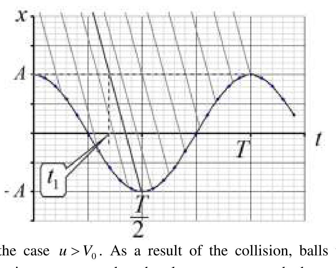
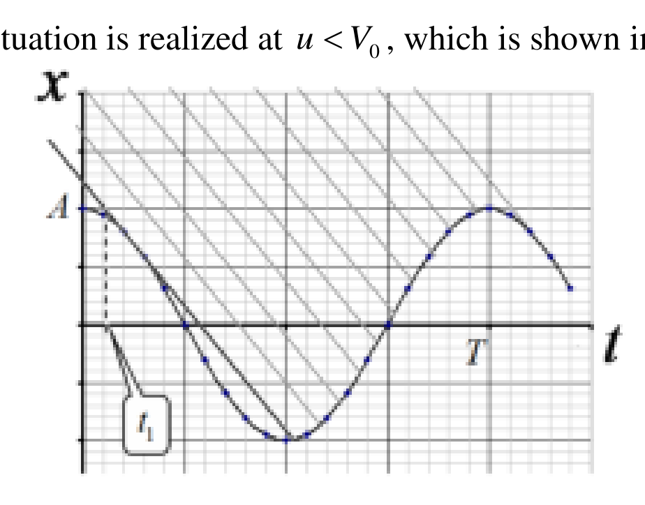
2.9 To answer the question posted, it is enough to consider one period of plate oscillations. Let us plot the dependence of the plate coordinates on time (22) and plot on the same graph the dependences of the incoming particle coordinates on time, which are straight lines $x = x_0 - ut$ .

The figure shows the case $u > V_0$ . As a result of the collision, balls that collide with the plate increase their speed at those time moments when the plate moves towards the positive direction of the axis , while collisions must occur in the time interval from $\frac{T}{2}$ to $T$ . However, the collision times are not randomly and uniformly distributed, but the times of approach to the plate itself are uniformly distributed, so we consider a plane $x = A$ , the times of approach to which are equally probable. Let us draw a straight line that describes the law of motion of a ball colliding with the plate at the moment of time $t = \frac{T}{2}$ (the thick line in the figure). Let us denote $t_1$ as the moment of time when this ball crosses the plane $x = A$ . Balls that collide with the plate after this moment of time increase their speed and energy. But these balls cross the plane in the time interval from $t_1$ to $T$ , so the fraction of these particles is obtained as

\eta = \frac{T - t_1}{T}. \qquad (25)

The moment of time $t_1$ is easy to find from the law of the ball motion

t_1 = \frac{T}{2} - \frac{2A}{u}, \qquad (26)

then the fraction of accelerated particles is equal to

\eta = \frac{T - t_1}{T} = \frac{1}{2} + \frac{2A}{uT} = \frac{1}{2} + \frac{V_0}{\pi u}. \qquad (27)

Here we use the relation that follows from formula (24): $\frac{2A}{T} = \frac{V_0}{\pi}$ . Substituting the specified numerical value $u = 1.5V_0$ , we get:

\eta = \frac{1}{2} + \frac{1}{1.5\pi} \approx 0.71. \qquad (28)

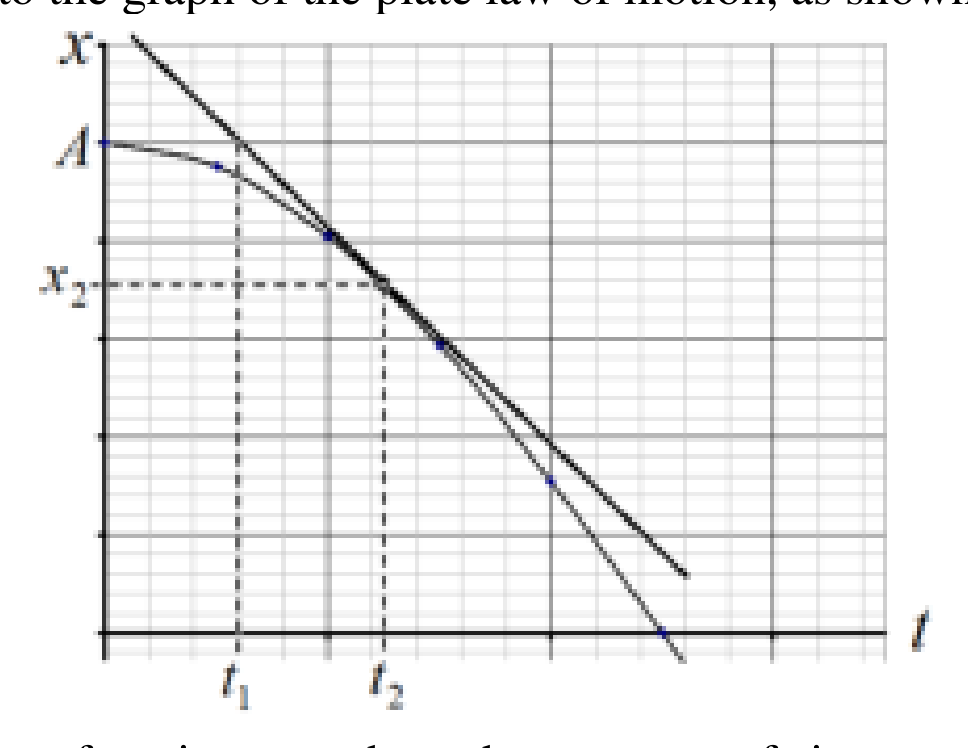
A somewhat different situation is realized at $u < V_0$ , which is shown in the figure below.

In this case, the "border time" $t_1$ between accelerated and decelerated balls is determined by a straight line, which is tangent to the graph of the plate law of motion, as shown in the figure below.

When the graphs of two functions touch at the moment of time $t_2$ , the values of both functions themselves and their derivatives, that is, the speeds of the plate and the ball, coincide, therefore

-A\omega\sin\left(\omega t_2\right) = -u, \qquad (29)

which gives rise to

t_2 = \frac{1}{\omega}\arcsin\frac{u}{A\omega} = \frac{T}{2\pi}\arcsin\frac{u}{V_0}. \qquad (30)

x_2 = A\cos\omega t_2 = A\sqrt{1 - \sin^2\omega t_2} = A\sqrt{1 - \frac{u^2}{V_0^2}}. \qquad (31)

These expressions allow us to determine the time of approach to the plane $x = A$

t_1 = t_2 - \frac{A - x_2}{u} = \frac{T}{2\pi}\left(\arcsin\frac{u}{V_0} - \frac{V_0}{u}\left(1 - \sqrt{1 - \frac{u^2}{V_0^2}}\right)\right). \qquad (32)

The ratio of this time to the oscillation period determines the fraction of particles that collide with the plate, catching it up, such that their energy decreases:

1 - \eta = \frac{1}{2\pi}\left(\arcsin\frac{u}{V_0} - \frac{V_0}{u}\left(1 - \sqrt{1 - \frac{u^2}{V_0^2}}\right)\right) \approx 0.04, \qquad (33)

therefore, the fraction of balls whose energy increases after the collision is equal to

\eta \approx 0.96. \qquad (34)

2.10 In one period of oscillation, the plate travels a path $4A$ , so the modulus of its speed is equal to

V = \frac{4A}{T}. \qquad (35)

2.11 When the ball speed is greater than the platform speed, the proportion of balls that increase their energy as a result of the collision is calculated by a formula similar to formula (27):

\eta = \frac{T - t_1}{T} = \frac{1}{2} + \frac{2A}{uT} = \frac{1}{2} + \frac{V}{2u}, \qquad (36)

and the corresponding figure is shown below.

Since the modulus of the plate velocity is assumed to be constant, the ball velocity modulus after the impact becomes equal to

u_+ = u + 2V. \qquad (37)

The velocities of balls that collide with the plate in the time interval from 0 to $t_1$ , are equal to

u_- = u - 2V. \qquad (38)

Thus, the average ball energy after the collision becomes equal to

\begin{aligned} E &= \eta\frac{mu_+^2}{2} + \left(1 - \eta\right)\frac{mu_-^2}{2} = \frac{m}{2}\left(\left(\frac{1}{2} + \frac{V}{2u}\right)\left(u + 2V\right)^2 + \left(\frac{1}{2} - \frac{V}{2u}\right)\left(u - 2V\right)^2\right) = \\ &= \frac{mu^2}{4}\left(\left(1 + \frac{V}{u}\right)\left(1 + 2\frac{V}{u}\right)^2 + \left(1 - \frac{V}{u}\right)\left(1 - 2\frac{V}{u}\right)^2\right) = \frac{mu^2}{2}\left(1 + 8\left(\frac{V}{u}\right)^2\right) \end{aligned}, \qquad (39)

and, consequently, the increase in the average energy is equal to

\varepsilon = 1 + 8\left(\frac{V}{u}\right)^2 \approx 4.6. \qquad (40)

If the speed of the balls is less than the speed of the plate, then all the balls collide with the plate when it moves in the opposite direction, so all the balls increase their speed and energy. After the collision, the particle velocities become equal $u_+ = u + 2V$ , and their energy

E = \frac{m}{2}\left(u + 2V\right)^2 = \frac{mu^2}{2}\left(1 + 2\frac{V}{u}\right)^2, \qquad (41)

and, consequently, the ratio of the ball energies after and before the collision is equal to

\varepsilon = \left(1 + 2\frac{V}{u}\right)^2 = 25.0. \qquad (42)

	Content	Points
2.1	Formula (2): $N_1 = n\Delta vt$	0.1	0.4
	Numerical value in formula (2): $N_1 \approx 0.83$	0.1
	Formula (3): $\tau_1 = \frac{1}{n\Delta v}$	0.1
	Numerical value in formula (3): $\tau_1 = 0.02\ \mathrm{h} = 72\ \mathrm{s}$	0.1
2.2	Formula (4): $N_2 = n\Delta vt$	0.1	0.4
	Numerical value in formula (4): $N_2 \approx 0.83$	0.1
	Formula (5): $\tau_2 = \frac{1}{n\Delta v}$	0.1
	Numerical value in formula (5): $\tau_2 = 0.02\ \mathrm{h} = 72\ \mathrm{s}$	0.1
2.3	Formulas (6): $N_{3,4} = n\left(2v \pm \Delta v\right)t$ , $\tau_{3,4} = \frac{1}{n\left(2v \pm \Delta v\right)}$	0.4	0.8
	Numerical values in formula (7): $N_3 = 14.2;\quad \tau_3 = 4.2\ \mathrm{s};$ $N_3 = 15.8;\quad \tau_3 = 3.8\ \mathrm{s}.$	0.4
2.4	Formula (8): $m_1v_1 + m_2v_2 = m_1u_1 + m_2u_2$	0.1	0.6
	Formula (9): $\frac{m_1v_1^2}{2} + \frac{m_2v_2^2}{2} = \frac{m_1u_1^2}{2} + \frac{m_2u_2^2}{2}$	0.1
	Formula (13): $u_1 = \frac{m_1 - m_2}{m_1 + m_2}v_1 + \frac{2m_2}{m_1 + m_2}v_2$	0,2
	Formula (14): $u_2 = \frac{2m_1}{m_1 + m_2}v_1 + \frac{m_2 - m_1}{m_1 + m_2}v_2$	0,2
2.5	Formula (15): $\eta_1 = \frac{1 - \mu}{1 + \mu} + \frac{2\mu}{1 + \mu}\eta_2$	0.2	1.6
	There are only straight lines on the graph, otherwise the graph is not graded	0.2
	All lines pass through the point $\eta_1 = 1; \eta_2 = 1$	0.4
	There is a straight line $\eta_1 = 1$	0.2
	There is a straight line $\eta_1 = -1 + 2\eta_2$	0.4
	All lines are located in between $\eta_1 = 1$ and $\eta_1 = -1 + 2\eta_2$	0,2
2.6	Inequalities (7): $\left\vert \eta_1\right\vert > 1 \Rightarrow \begin{cases} \eta_1 > 1 \\ \eta_1 < -1 \end{cases}$	0.2	0.4
	Inequality (19): $\eta_2 > 1$	0.1
	Inequality (20): $\eta_2 < -\frac{1}{\mu}$	0.1
2.7	Formula (21): $\tilde{u}_1 = -v_1 + 2v_2$	0.1	0.3
	Inequality a): $v_2 > 1$	0.1
	Inequality b): $v_2 < 0$	0.1
2.8	Formula (22): $x(t) = A\cos(\omega t)$	0.1	0.4
	Formula (23): $v(t) = -A\omega\sin(\omega t)$	0.1
	Formula (24): $V_0 = A\omega = 2\pi\frac{A}{T}$	0,2
2.9	Formula (25): $\eta = \frac{T - t_1}{T}$	0.3	2.7
	Formula (26): $t_1 = \frac{T}{2} - \frac{2A}{u}$	0.3
	Formula (27): $\eta = \frac{1}{2} + \frac{V_0}{\pi u}$	0.3
	Numerical value in formula (28): $\eta \approx 0.71$	0.3
	Formula (29): $-A\omega\sin\left(\omega t_2\right) = -u$	0.2
	Formula (30): $t_2 = \frac{T}{2\pi}\arcsin\frac{u}{V_0}$	0.2
	Formula (31): $x_2 = A\sqrt{1 - \frac{u^2}{V_0^2}}$	0.3
	Formula (32): $t_1 = \frac{T}{2\pi}\left(\arcsin\frac{u}{V_0} - \frac{V_0}{u}\left(1 - \sqrt{1 - \frac{u^2}{V_0^2}}\right)\right)$	0.3
	Formula (33): $1 - \eta = \frac{1}{2\pi}\left(\arcsin\frac{u}{V_0} - \frac{V_0}{u}\left(1 - \sqrt{1 - \frac{u^2}{V_0^2}}\right)\right)$	0.3
	Numerical value in formula (34): $\eta \approx 0.96$	0.2
2.10	Formula (35): $V = \frac{4A}{T}$	0.2	0.2
2.11	Formula (36): $\eta = \frac{1}{2} + \frac{V}{2u}$	0.3	2.2
	Formula (37): $u_+ = u + 2V$	0.2
	Formula (38): $u_- = u - 2V$	0.2
	Formula (39): $E = \eta\frac{mu_+^2}{2} + \left(1 - \eta\right)\frac{mu_-^2}{2}$	0.3
	Formula (40): $\varepsilon = 1 + 8\left(\frac{V}{u}\right)^2$	0.3
	Numerical value in formula (40): $\varepsilon \approx 4.6$	0.2
	Formula (41): $E = \frac{m}{2}\left(u + 2V\right)^2$	0.2
	Formula (42): $\varepsilon = \left(1 + 2\frac{V}{u}\right)^2$	0.3
	Numerical value in formula (42): $\varepsilon = 25.0$	0.2
Total			10.0

Graph of x versus t for the case u > V0: the plate coordinate is a cosine curve starting at A, reaching −A at T/2 and returning to A at T; many parallel descending straight lines are ball trajectories; the thick line touches the plate at t = T/2 and crosses the dashed level x = A at the time marked t1 by a callout.

Graph of x versus t for the case u < V0: a cosine plate curve starting at A with minimum near T/2 and maximum at T; parallel descending ball trajectories; one line is tangent to the plate curve on its descending branch, and the dashed vertical line at the time where it crosses x = A is marked t1 by a callout.

Enlarged graph of x versus t near the start: the plate curve descends from A and a straight ball trajectory touches it at time t2 at the height x2 (dashed lines to both axes); the same straight line crosses the level x = A at time t1, also marked with a dashed vertical line.

Graph of x versus t for the piecewise-linear plate motion: a zigzag from A down to −A and back up to A at T; parallel descending ball trajectories; a thicker trajectory meets the plate at its lowest point −A, and a callout marks t1 near the t axis.

Mathematical hints for the theoretical problems

The following formulas may be useful:

$\displaystyle\int x^n dx = \frac{x^{n+1}}{n+1} + C$ , where $n \neq -1$ is a fixed number, $C$ refers to an arbitrary constant;

$\displaystyle\int \frac{dx}{x} = \ln|x| + C$ , where $C$ stands for an arbitrary constant;

$\displaystyle\int \frac{dx}{(x^2 + a^2)^{3/2}} = \frac{x}{a^2(x^2 + a^2)^{3/2}} + C$ , where $a, C$ stand for arbitrary constants;

$\displaystyle(1 + x)^{\gamma} \approx 1 + \gamma x + \frac{\gamma(\gamma - 1)}{2}x^2$ , for $|x| \ll 1$ and arbitrary $\gamma$ ;

$\ln(1 + x) \approx x$ , for $|x| \ll 1$ .

Оригинал в Архива: IZhO 2023 PhysTheory_eng.pdf · официални решения: IZhO-2023-Theory_multi_sol.pdf