Съдържание

Условие Отговори Решение

IZhO 2024, Експеримент — Задача 1. Superposition of oscillations

Оригинал на условието (PDF)Съобщи за грешка

Всички материали от IZhO 2024

XX International Zhautykov Olimpiad/Experimental Competition · 10 януари 2024 г. · 20 т.

Please read the instructions first:

EXPERIMENTAL COMPETITION

January 10, 2024

The Experimental competition consists of one problem. This part of the competition lasts 3 hours.
Please only use the pen that is provided to you.
You can use your own non-programmable calculator for numerical calculations. If you don’t have one, please ask for it from Olympiad organizers.
You are provided with Writing sheet and additional papers. You can use the additional paper for drafts of your solutions but these papers will not be checked. Your final solutions which will be evaluated should be on the Writing sheets. Please use as little text as possible. You should mostly use equations, numbers, figures and plots.
Use only the front side of Writing sheets. Write only inside the bordered area.
Fill the boxes at the top of each sheet of paper with your country (Country), your student code (Student Code), the question number (Question Number), the progressive number of each sheet (Page Number), and the total number of Writing sheets (Total Number of Pages). If you use some blank Writing sheets for notes that you do not wish to be evaluated, put a large X across the entire sheet and do not include it in your numbering.
At the end of the exam, arrange all sheets for each problem in the following order:
- Used Writing sheets in order.
- The sheets you do not wish to be evaluated.
- Unused sheets.
- The printed problems.
Place the papers inside the envelope and leave everything on your desk. You are not allowed to take any paper or equipment out of the room.

Условие

Devices and equipment: tripod, complex pendulum, ruler of 30 cm, electronic stopwatch.

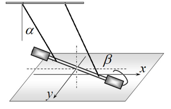
The oscillatory system is a torsion pendulum, which consists of a metal screw-threaded rod 1, suspended on two threads 2 and 3 of equal length, the threads are tied to a horizontal rod 4, fixed in the tripod leg. On the movable rod 1 there are two elongated screw nuts 5 and 6, which can be freely moved along the rod.

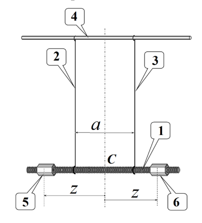
Schematic of the pendulum: a horizontal rod 4 at the top; two vertical threads 2 and 3 at distance a hang from it and hold the screw-threaded rod 1 with centre C; two nuts 5 and 6 sit on the rod at distance z on either side of the centre; a dash-dotted vertical line marks the axis of symmetry.

In all experiments, the lengths of the threads must remain unchanged, and they themselves must be strictly vertical in a state of equilibrium and located symmetrically relative to the center of the rod $C$ . We denote the distance between the threads as $a$ .

The screw nuts should also be positioned symmetrically relative to the center of the rod. The position of the nuts is determined by the distance $z$ from the rod center to the middle of the nut. For precise positioning of the nuts, it is recommended to use a rod thread with a pitch of 1.0 mm. For convenience, one of the faces of the nut is sealed with a strip of paper on which its middle is clearly marked, so that when the nut is turned one turn, it moves along the rod by a distance of 1.0 mm.

In this experiment you need to study two types of the rod oscillations:

longitudinal oscillations (1 in the figure below), in which the rod and threads always move in the same vertical plane;
torsional oscillations (2 in the figure below), in which the rod rotates around a fixed vertical axis passing through the rod center.

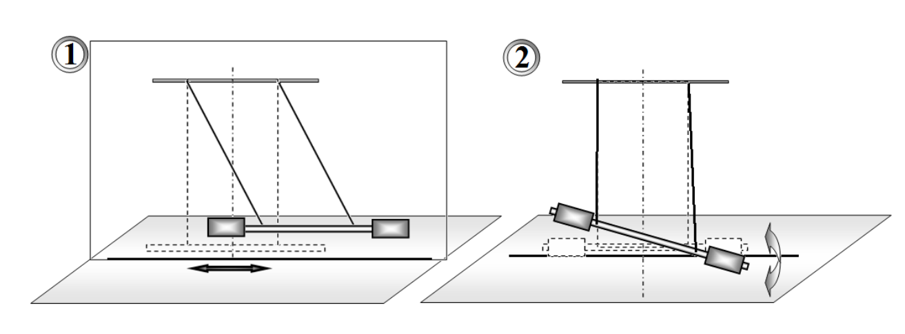
Two perspective sketches of the pendulum above a sheet of paper. Sketch 1: the threads are tilted in the vertical plane of the rod, the rod is displaced along its axis, a double arrow shows the longitudinal motion. Sketch 2: the rod is rotated about the vertical axis through its centre, a curved arrow shows the torsional motion; the equilibrium position is dashed.

If the rod is deflected in a vertical plane and released, it then performs longitudinal oscillations. If the rod is rotated at a certain angle around the vertical axis and released, it then performs torsional oscillations.

In addition, this experiment is aimed at studying the superposition of longitudinal and torsional oscillations, which can be excited by displacing the rod along its axis and rotating it at a certain angle relative to the vertical axis. We call such oscillations mixed.

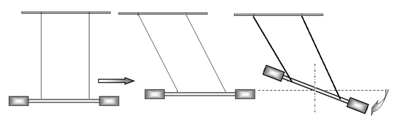
Three sketches showing how mixed oscillations are excited: the pendulum at rest; an arrow; the rod displaced along its axis with inclined threads; then the rod additionally rotated about the vertical axis, with a curved arrow.

For convenience, secure the pendulum in a tripod so that the rod moves in close proximity to the table surface. Place a sheet of paper on the table, on which you have to draw a straight line corresponding to the rod equilibrium position. During longitudinal oscillations, the rod must move along this straight line; during torsional oscillations, the center of the rod must be located on the same vertical.

During the experiments, the angles of deviation of the threads from the vertical during longitudinal oscillations and the angles of rod rotation during torsional oscillations should lie in the range of 20°-30°.

Successful completion of this experiment requires high precision measurements, so be extremely careful and accurate! Release the rod without any additional push!

Part 1. Observation of the effect and its theoretical description

Place the threads at a distance of $a = 20$ cm, their lengths should approximately be $L = 45$ cm, and the screw nuts should be placed at the ends of the movable rod. Excite mixed oscillations of the rod and carefully observe the movement of one of its ends. Since, with the selected system parameters, the frequencies of longitudinal and torsional oscillations are close, the shape of the trajectory of the rod end changes slowly and regularly, periodically returning to the initial one. Let us call the process of sequential restoration of the original shape of the trajectory a cycle, the corresponding time as the cycle time $T_C$ , and the number of complete longitudinal oscillations corresponding to it as $N_C$ .

1.1 Draw several successive characteristic shapes of the rod end trajectories in one cycle. [1 т.]

We introduce a coordinate system on the horizontal plane: the $x$ axis is directed along the rod in the position of its equilibrium, the $y$ axis is perpendicular to it, and the origin is placed under the center of the rod in the position of its equilibrium.

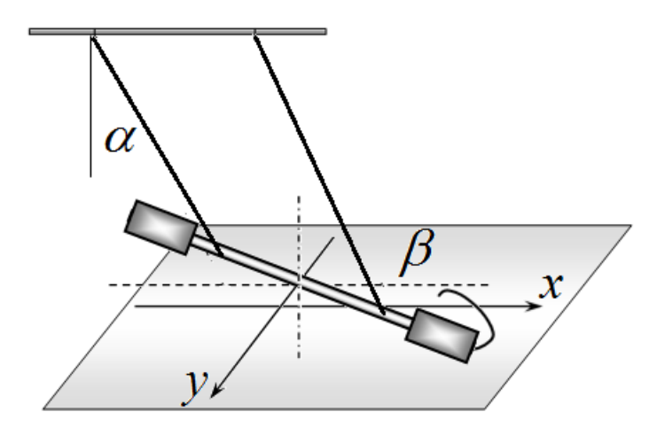
Perspective sketch of the deflected pendulum above a horizontal plane with the coordinate axes x (along the rod in equilibrium) and y (perpendicular); the thread deflection angle α from the vertical and the rod rotation angle β are marked.

We also denote the angle of deflection of the threads during longitudinal oscillations as $\alpha$ , the angle of rod rotation during torsional oscillations as $\beta$ , the period of longitudinal oscillations as $T_0$ , the period of torsional oscillations as $T_1$ , the length of the threads as $L$ , and the length of the rod as $l$ .

1.2 Write down the exact dependences of the coordinates of the rod end $x(t)$ and $y(t)$ on time $t$ , and then obtain the corresponding approximate expressions for the conditions of this experiment. [0,8 т.]

1.3 Within the framework of the proposed model, obtain a formula for the cycle period $T_C$ , expressing it through the periods of longitudinal $T_0$ and torsional $T_1$ oscillations. [1,3 т.]

1.4 Write down the formula for the number of longitudinal oscillations in the cycle $N_C$ , expressing it in terms of periods $T_0$ and $T_1$ . [0,4 т.]

Part 2. Longitudinal oscillations

2.1 Measure the period of longitudinal oscillations $T_0$ with the possible minimal error. Calculate the instrumental, random and total errors of the measured value of the period $\Delta T_0$ . [2 т.]

Part 3. Torsional oscillations

The period of torsional oscillations can be described by the formula:

\frac{T_1}{T_0} = a^q F(z), \qquad (1)

where $z$ signifies the distance from the rod center to the centers of the nuts, and $F(z)$ stands for a function that depends on $z$ only.

3.1 Measure the dependence of the period of torsional oscillations $T_1$ on the distance between the threads $a$ , plot a graph of the resulting dependence. Take measurements when the nuts are at the rod ends with $z = 17$ cm. [2,5 т.]

3.2 Based on experimental data, prove the validity of formula (1) and determine the exponent $q$ . An error estimate is not required here. [1,5 т.]

It can be shown that the function $F(z)$ in formula (1) has the following form

F(z) = \sqrt{A + Bz^2}, \qquad (2)

where $A, B$ refer to some constant values independent of the parameters $a$ and $z$ .

3.3 Fix the suspension threads at a distance of $a = 10$ cm. Measure the period of torsional oscillations as a function of the position of the nuts $z$ . Plot a graph of the resulting relationship. It is unnecessary to take measurements when the nuts are closer to the center of the rod than the threads. [2,5 т.]

3.4 Prove the applicability of formula (2) to describe your experimental data. [1 т.]

3.5 Calculate the values of the coefficients $A, B$ and estimate their errors. Please note that $a, z$ values must be measured in centimeters. [1 т.]

Part 4. Mixed oscillations

Place the threads at a distance of $a = 20$ cm. Investigate the mixed oscillations described in Part 1 for different positions of the nuts with $z > 10$ cm.

4.1 Measure the dependence of the number of longitudinal oscillations in the cycle $N_C$ on the position of the nuts $z$ . You may not be able to do this for all $z$ values! [4 т.]

4.2 Based on the results of parts 2 and 3, calculate the periods of torsional oscillations for all values of $z$ at which the measurements have carried out in section 4.1. [0,5 т.]

4.3 Present the measurement results in such a graphical form that they confirm the validity of the formula for the $N_C$ value obtained in part 1. [1,5 т.]

Отговори

Решение

SOLUTION TO THE EXPERIMENTAL COMPETITION

Superposition of oscillations

The longitudinal and torsional oscillations of the pendulum described in the experiment in the approximation of small angles are its own oscillations (modes), so they can be considered independently of each other.

In the small angle approximation, the periods of these oscillations are given by the formulas

T_0 = 2\pi\sqrt{\frac{L}{g}}, \qquad (1)

T_1 = 2\pi\sqrt{\frac{4LI}{mga^2}}, \qquad (2)

where $m = m_0 + 2m_1$ is the total mass of the pendulum, $m_0$ refers to the rod mass, $m_1$ stands for the nut mass, and $I = \frac{m_0 l^2}{12} + 2m_1 z^2$ designates the moment of inertia of the rod with the nuts.

Formulas (1) and (2) are actually used in the work, but their derivation is not required and is not graded.

Part 1. Observation of the effect and its theoretical description

1.1 The rod end moves along trajectories corresponding to the addition of perpendicular oscillations with close frequencies. They can also be thought of as the addition of oscillations with equal frequencies, but with a slowly varying phase difference between them. Images of these most typical trajectories are shown in the figure below.

Five dashed frames showing successive trajectories of the rod end in one cycle: an inclined segment with arrows at both ends, a clockwise ellipse, a segment inclined the other way, a counter-clockwise ellipse, and again the first inclined segment.

1.2 It follows from geometry that the horizontal coordinates of the rod end are described by the formulas:

\begin{cases} x = L\sin\alpha + \frac{l}{2}\cos\beta \\ y = \frac{l}{2}\sin\beta \end{cases}. \qquad (3)

Perspective sketch of the deflected pendulum above a horizontal plane with axes x and y; the thread deflection angle α and the rod rotation angle β are marked.

In the approximation of small angles $\alpha, \beta \ll 1$ we have

\begin{cases} x \approx L\alpha + \frac{l}{2} \\ y \approx \frac{l}{2}\beta \end{cases}. \qquad (4)

Since the angles $\alpha, \beta$ change according to a harmonic law with frequencies $\omega_0 = 2\pi/T_0$ and $\omega_1 = 2\pi/T_1$ , respectively, the equation for the trajectory of the rod end has the form

\begin{cases} x(t) = L\alpha_{max}\cos\omega_0 t + \frac{l}{2} \\ y(t) = \frac{l}{2}\beta_{max}\sin\omega_1 t \end{cases}, \qquad (5)

which for close frequencies can be conveniently rewritten in the form

\begin{cases} x(t) = L\alpha_{max}\cos\omega_0 t + \frac{l}{2} \\ y(t) = \frac{l}{2}\beta_{max}\sin(\omega_0 t + (\omega_1 - \omega_0)t) \end{cases}. \qquad (6)

In the expression $y(t)$ for close frequencies, the value $\Delta\varphi = (\omega_1 - \omega_0)t$ can be considered as a slowly varying phase difference between oscillations with close frequencies.

1.3 It is obvious that the shape of the trajectory returns to the initial one if the phase difference changes by $\pm 2\pi$ . Thus, the cycle period obeys the condition

(\omega_1 - \omega_0)T_C = \pm 2\pi, \qquad (7)

which provides

T_C = \frac{T_0 T_1}{|T_0 - T_1|}. \qquad (8)

1.4 The number of oscillations of longitudinal oscillation in the cycle can be written in the form

N_C = \frac{T_C}{T_0} = \frac{T_1}{|T_0 - T_1|}. \qquad (9)

Part 2. Longitudinal oscillations

2.1 To increase the measurement accuracy, it is necessary to measure the times of a sufficiently large number of oscillations; in our experiments, we measure the time of 20 periods of oscillations $t_{20}$ . To estimate the random error, these measurements are carried out 10 times, and their results are shown in Table 1.

Table 1. Measuring the period of longitudinal oscillations.

$n$	$t_{20}$ , s
1	26,39
2	26,32
3	26,51
4	26,40
5	26,46
6	26,41
7	26,34
8	26,22
9	26,55
10	26,53

The average time of 20 oscillations is
$\langle t_{20} \rangle = 26.41$ s, and the instrument error is equal to half the value of the stopwatch division
$\Delta t_1 = 0.5 \cdot 10^{-3}$ s.
The random error is calculated using the formula

\Delta t_2 = 2\sqrt{\frac{\sum_{i=1}^{10}\left(t_{20,i} - \langle t_{20} \rangle\right)^2}{n(n-1)}} = 6.5 \cdot 10^{-2}\ \mathrm{s}.

The total time measurement error is
$\Delta t = \sqrt{\Delta t_1^2 + \Delta t_2^2} = 0.066$ s.

Thus, the period of longitudinal oscillations is equal to

T_0 = \frac{t_{20}}{20} = (1.321 \pm 0.003)\ \mathrm{s}. \qquad (10)

Part 3. Torsional oscillations

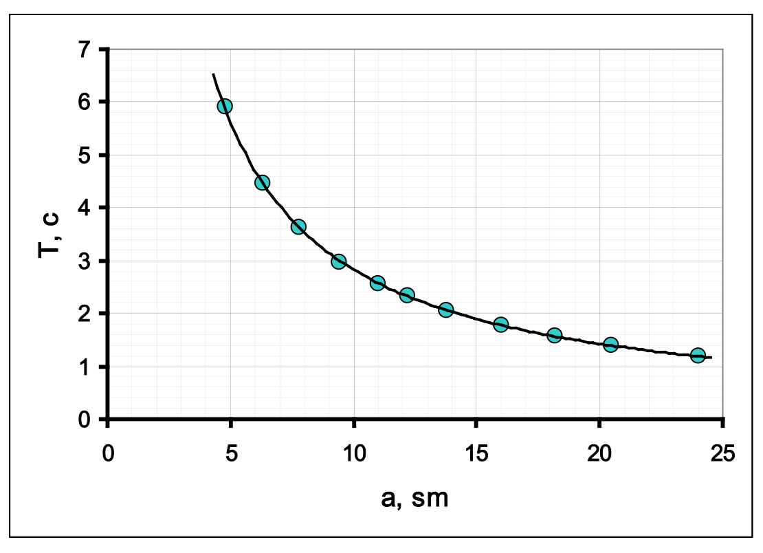
3.1 Table 2 shows the values of the measurement results of the periods of torsional oscillations at various values of the distance $a$ between the threads. The same table shows the results of calculations for determining the exponent $q$ .

Table 2. Dependence of the period of torsional oscillations as a function of the distance between the threads.

$a$ , cm	$t_{10}$ ,s	$T_1$ , s	$\ln a$	$\ln T_1$
4,8	59,11	5,911	1,5686	1,7768
6,3	44,62	4,462	1,8405	1,4956
7,8	36,31	3,631	2,0541	1,2895
9,4	29,66	2,966	2,2407	1,0872
11,0	25,60	2,560	2,3979	0,9400
12,2	23,32	2,332	2,5014	0,8467
13,8	20,46	2,046	2,6247	0,7159
16,0	17,66	1,766	2,7726	0,5687
18,2	15,82	1,582	2,9014	0,4587
20,5	13,87	1,387	3,0204	0,3271
24,0	11,98	1,198	3,1781	0,1807

The corresponding dependence graph looks like

Graph of the torsional period T, c (0–7) versus the thread distance a, sm (0–25): measured points on a smooth decreasing hyperbola-like curve from about 5.9 at a = 4.8 to about 1.2 at a = 24.

3.2 The optimal and most common way to determine the exponent is to plot a graph on a double logarithmic scale. It follows from formula (1) given in the problem statement that

\ln T = C + q\ln a, \qquad (11)

therefore, the slope of the graph is equal to the exponent. This graph is shown in the figure below.

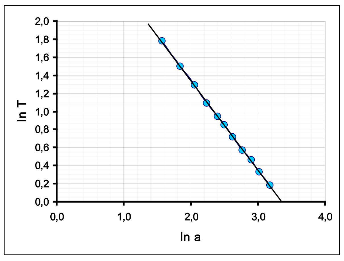
Graph of ln T (0,0–2,0) versus ln a (0,0–4,0): the measured points lie on a falling straight line with slope close to −1, from about (1,57; 1,78) to (3,18; 0,18).

The resulting relationship is linear with a slope coefficient very close to (-1). An alternative way is to construct dependencies $T_1(a^{-1})$ , or $T_1^{-1}(a)$ . However, in these methods it is necessary to prove that the constructed graphs are straight lines passing through the origin of coordinates.

All these methods reasonably indicate that the desired exponent is equal to (-1), i.e. the period of torsional oscillations is inversely proportional to the distance between the threads.

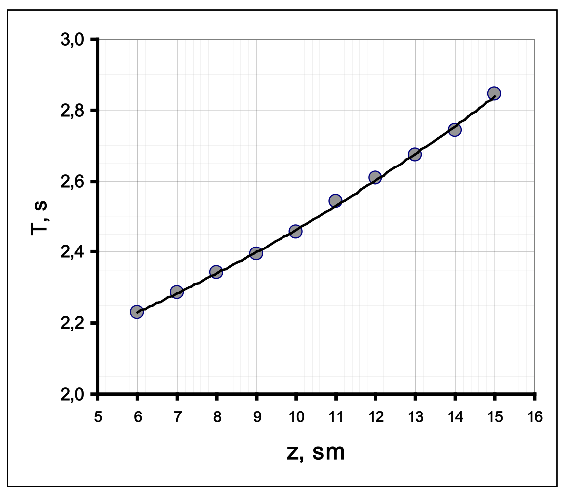
3.3 The results of measurements of the dependence of the period of torsional oscillations on the position of the nuts are given in Table 3. The same table shows the calculation results necessary to construct a linearized graph.

Table 3. Measurements of the period of torsional oscillations.

$z$ , cm	$t_{20}$ , s	$T_1$ , s	$z^2$	$T_1^2$	$U$
6	44,58	2,229	36	4,968	284,9
7	45,75	2,288	49	5,233	300,0
8	46,83	2,342	64	5,483	314,3
9	47,87	2,394	81	5,729	328,5
10	49,17	2,459	100	6,044	346,5
11	50,84	2,542	121	6,462	370,5
12	52,15	2,608	144	6,799	389,8
13	53,47	2,674	169	7,148	409,8
14	54,85	2,743	196	7,521	431,2
15	56,91	2,846	225	8,097	464,2

The graph of this relationship is shown in the figure below. It can be seen that the resulting dependence is nonlinear.

Graph of T, s (2,0–3,0) versus z, sm (5–16): the measured points from z = 6 to z = 15 rise from about 2,23 to 2,85 along a slightly curved line.

3.4 It follows from formulas (1)-(2) given in the problem statement and the result of the previous part that the period of torsional oscillations is described by the formula

\frac{T_1}{T_0} = \frac{\sqrt{A + Bz^2}}{a}, \qquad (12)

whose linearization is obvious and has the form

\left(a\frac{T_1}{T_0}\right)^2 = A + Bz^2. \qquad (13)

The value $U = \left(a\frac{T_1}{T_0}\right)^2$ depends linearly on $z^2$ , and the graph of the linearized dependence is shown in the figure below.

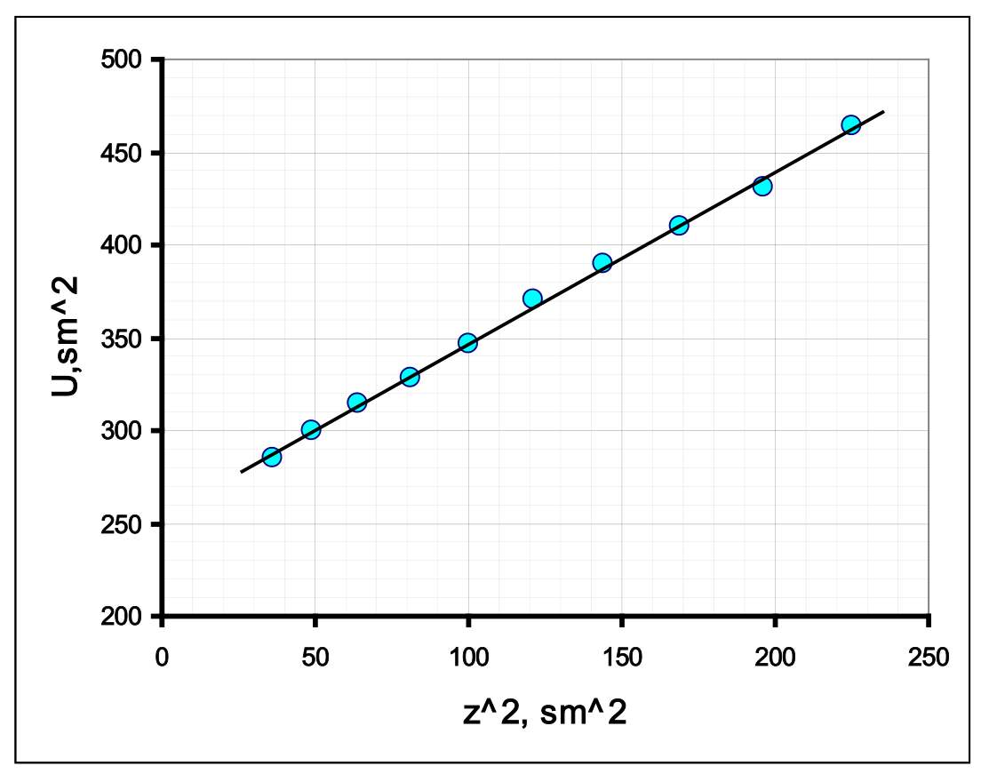
Graph of U, sm^2 (200–500) versus z^2, sm^2 (0–250): the measured points from about (36; 285) to (225; 464) lie on a rising straight line.

3.5 The coefficients of this dependence, calculated using the least squares method, are equal to

A = (254 \pm 4)\ \mathrm{cm}^2, \qquad (14)

B = 0.93 \pm 0.03. \qquad (15)

Part 4. Mixed oscillations

4.1, 4.2 Table 4 shows the results of measurements and calculations necessary to verify the theoretical formula (9).

Table 4. Study of mixed oscillations.

$z$ , cm	$T_1$ , s	$\frac{T_0}{T_1}$	$N_C$ (теор.)	$N_C$ (эксп)	$\frac{1}{N_C}$
10,5	1,247	1,059	17
11,0	1,264	1,045	22	24	0,042
11,5	1,282	1,030	33	35	0,029
12,0	1,301	1,015	65
12,5	1,319	1,002	660
13,0	1,339	0,987	74	60	0,017
13,5	1,359	0,972	36	33	0,030
14,0	1,379	0,958	24	21	0,048
14,5	1,400	0,944	18	16	0,063
15,0	1,421	0,930	14	13	0,077

In this table $T_1$ stands for values of torsional oscillation periods calculated using formula (12), and $N_C$ refers to the calculated and measured values of the number of periods in the cycle.

4.3 To check formula (9), a graph is drawn of the dependence of the quantity reciprocal to the number of oscillations $\frac{1}{N_C}$ on the value $\frac{T_0}{T_1}$ , which is theoretically described by the formula $\frac{1}{N_C} = \left|\frac{T_0}{T_1} - 1\right|$ . A graph of this dependence, constructed from the experimental data, is shown in the figure below.

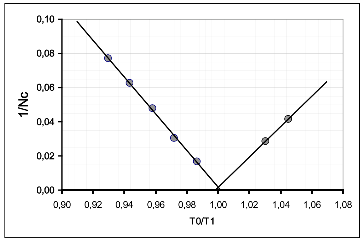
Graph of 1/Nc (0,00–0,10) versus T0/T1 (0,90–1,08): a V-shaped pair of straight lines with the minimum at T0/T1 = 1,00; five measured points lie on the left branch and two on the right branch.

This graph, as well as a comparison of the calculated and measured $N_C$ values, corroborates the theoretical conclusions.

	Content	Points	Total
	Part 1. Observation of the effect and its theoretical description
1.1	The addition of vibrations is obtained (there is at least one plausible picture)	0,2	1,0
	4 drawings: two close to the segment, two ovals indicating the direction of motion	4x0,2=0,8
1.2	Expressions for coordinates on a plane through deflection angles	2x0,2=0,4	0,8
	Explicit time dependencies	2x0,1=0,2
	Small angle approximation	0,2
1.3	The main idea is the change in phase difference, formula (7); (if the beat period)	0,5 (0,2)	1,3
	Formula (8) for the cycle time	0,5
	The module is placed in formula (8)	0,3
1.4	$N_C = \frac{T_1}{\lvert T_0 - T_1 \rvert}$ .	0,4	0,4
	Part 2. Longitudinal oscillations
	Graded if the numerical value of the oscillation period is estimated
2.1	The obtained period value is in the range of 1.3 – 1.5 s	0,4	2,0
	Measurement error less than 1% (graded if the error is estimated)	0,1
	At least 5 measurements of time N oscillations were carried out (3, less)	0,3 (0,1;0)
	Number of oscillations N not less than 10 (5; less)	0,2 (0,1;0)
	Averaging over all measurements are carried out	0,1
	Random error calculated (averaging of deviation modules, standard deviation - acceptable)	0,2
	Instrument error (half or division value)	0,2
	The total error is calculated (the value is acceptable)	0,2
	Correct rounding (error – 1-2 digits, result – up to the error digit)	0,2
	The dimension of the result is indicated	0,1
	Part 3. Torsional oscillations
	Graded if the measurement results are graded!
3.1	If the nuts are not located at the ends of the rod, the grades are divided by factor 2.		2,5
	For each measurement 0.15 (in total no more than 1.5; falling within the 20% range if the time of less than 10 oscillations is measured, 0.1 per measurement)	0,15x10=1,5
	The lower limit of the range is no more than 5.0 cm	0,2
	The upper limit of the range is not less than 15.0 cm	0,2
	A nonlinear dependence close to hyperbolic is obtained	0,1
	Plotting a graph (the axes are labeled and digitized, all points are plotted in accordance with the table, a smoothing curve is drawn)	0,1+0,2+0,2= =0,5
3.2	Graded if the degree is -1, the measurement results are graded		1,5
	The obtained value is q=-1	0,5
	Linearization is carried out on a double logarithmic scale (calculations are provided) (reciprocals, with proof of passing through zero);	0,5 (0,2+0,2)
	A graph of the linearized dependence is plotted (the axes are labeled and digitized, all points are plotted in accordance with the table, a smoothing line is drawn)	0,1+0,2+0,2= =0,5
3.3	If the distance between the threads is different from 10 cm, the grades are divided by factor 2		2,5
	For each measurement 0.15 (in total no more than 1.5; falling within the 20% range if the time of less than 10 oscillations is measured, 0.1 per measurement)	0,15x10=1,5
	The lower limit of the range is no more than 6.5 cm	0,2
	The upper limit of the range is not less than 14.0 cm	0,2
	A nonlinear downward convexity dependence is obtained	0,1
	A graph of the linearized dependence is plotted (the axes are labeled and digitized, all points are plotted in accordance with the table, a smoothing line is drawn)	0,1+0,2+0,2= =0,5
3.4	Linearization is carried out (the squares of periods and distances are calculated)	0,3	1,0
	A graph of linearized dependence is plotted (the axes are labeled and digitized, all points are plotted in accordance with the table, a smoothing line is drawn)	0,1+0,2+0,2= =0,5
	Straight line is obtained	0,2
3.5	Grades if 3.3 – 3.4 are graded		1
	Numerical values of the coefficients are obtained (in the range of 20%, the dimension -0.1 is not indicated)	2x0,4=0,8
	Errors of coefficients are calculated	2x0,1=0,2
	Calculation using LSM coefficient 1; graphically, averaging over all points – 0.8; at two points – 0.5;
	Part 4. Mixed oscillations
	Graded if measurement results are graded
4.1	For each measurement 0.2 (total no more than 2.0; within 30% range)	0,2x10=2,0	4
	There are two dependency branches (at least 2 points on each)	1,0
	The lower limit of the range is no more than 11 cm	0,2
	The upper limit of the range is at least 15 cm	0,2
	The number obtained N>50	0,3
	Sharp increase (steeper than linear)	0,1
	There is an "unmeasured" area in the middle of the range	0,2
4.2	The periods are calculated (range – 20%) at 0.05 for each point, at least 3 decimal places)	0,05x10=0,5	0,5
4.3	Linearization is proposed (the reciprocal of the number of oscillations from the ratio of periods, the difference of periods); A theoretical calculation of the number of oscillations are carried out and a comparison with experimental results is made.	0,5 0,2+0,1=0,3	1,5
	The linearized dependence is calculated	0,2
	A graph of linearized dependence is plotted A graph of measurement results is plotted	0,4 0,2
	A graph similar to the graph of the modulus number function is obtained	0,3
	Correct position of the minimum on the graph	0,1
	TOTAL		20,0

Оригинал в Архива: IZhO-2024-Exp_eng.pdf · официални решения: IZhO-2024-Exp_multi_sol.pdf