Съдържание

USAAAO 2024, II кръг — Long 1. TESS

Оригинал на условието (PDF)Съобщи за грешка

Всички материали от USAAAO 2024

2024 National Astronomy Competition · 50 т.

Внимание: Бележка към темата

All eight whole original problems, their native sections, lettered parts, three roman subparts of Long 1(f), full official worked keys and original marking/acceptance notes are retained. Printed scientific discrepancies are preserved in local source notes. The official key adds a Friedmann-variable clarification and a solar apparent magnitude assumption absent from the question booklet, and changes Long1(f)(iii) from a factor to a percentage; these source variants are explicitly attributed. A separate undated common archive constants/reference table is included with its own source identity; its use as the exact 2024 provided attachment is not established, and its constants are not substituted into the printed key. The native cover specifies blank paper rather than a designated answer sheet. April 13th is the end of the examination period, not an established single sitting date.

1 Instructions (Please Read Carefully)

The top 5 eligible scorers on the NAC will be invited to represent USA at the next IOAA. In order to qualify for the national team, you must be a high school student with US citizenship or permanent residency.

This exam consists of 3 parts: Short Questions, Medium Questions and Long Questions.

The maximum number of points is 225 points.

The test must be completed within 2.5 hours (150 minutes).

Please solve each problem on a blank piece of paper and mark the number of the problem at the top of the page. The contestant’s full name in capital letters should appear at the top of each solution page. If the contestant uses scratch papers, those should be labeled with the contestant’s name as well and marked as “scratch paper” at the top of the page. Scratch paper will not be graded. Partial credit will be available given that correct and legible work was displayed in the solution.

This is a written exam. Contestants can only use a scientific or graphing calculator for this exam. A table of physical constants will be provided. Discussing the problems with other people is strictly prohibited in any way until the end of the examination period on April 13th. Receiving any external help during the exam is strictly prohibited. This means that the only allowed items are: a calculator, the provided table of constants, a pencil (or pen), an eraser, blank sheets of papers, and the exam. No books or notes are allowed during the exam. Exam is proctored and recorded. You are expected to have your video on at all times.

We acknowledge the following people for their contributions to this year’s exam:

Abhay Bestrapalli, Orion Foo, Hagan Hensley, David Lee, Sandesh Kalantre, Andrew Liu, Joe McCarty, Leo Yao

Common archive reference — Table of Physical Constants

This separate common USAAAO archive reference is undated in the catalogue. Its use as the exact 2024 exam attachment is not established.

Quantity	Symbol	Value
Electron rest mass	$m_e$	$9.109\times10^{-31}\ \mathrm{kg}$
Proton rest mass	$M_p$	$1.6726\times10^{-27}\ \mathrm{kg}$
Electronic charge	$e$	$1.6022\times10^{-19}\ \mathrm C$
Speed of light in free space	$c$	$2.9979\times10^8\ \mathrm{m\ s^{-1}}$
Permeability of free space	$\mu_0$	$4\pi\times10^{-7}\ \mathrm{H\ m^{-1}}$
Permittivity of free space	$\epsilon_0$	$8.854\times10^{-12}\ \mathrm{F\ m^{-1}}$
Planck’s constant	$h$	$6.626\times10^{-34}\ \mathrm{J\ s}$
Reduced Planck’s constant	$\hbar=h/2\pi$	$1.0546\times10^{-34}\ \mathrm{J\ s}$
	$\hbar c$	$197.33\ \mathrm{MeV\ fm}$
Boltzmann’s constant	$k_B$	$1.3807\times10^{-23}\ \mathrm{J\ K^{-1}}$
Gas constant	$\mathcal R=k_B/m_H$	$8.250\times10^3\ \mathrm{J\ kg^{-1}\ K^{-1}}$
Molar gas constant	$R$	$8.315\ \mathrm{J\ mol^{-1}\ K^{-1}}$
Avogadro’s number	$N_A$	$6.022\times10^{23}\ \mathrm{mol^{-1}}$
Standard molar volume		$22.414\times10^{-3}\ \mathrm{m^3\ mol^{-1}}$
Unified atomic mass unit ( $^{12}\mathrm C$ scale)	$u$	$931.5\ \mathrm{MeV}/c^2=1.660538\times10^{-27}\ \mathrm{kg}$
Mass of hydrogen atom	$m_H$	$1.0078u=1.6735\times10^{-27}\ \mathrm{kg}$
Bohr magneton	$\mu_B$	$9.274\times10^{-24}\ \mathrm{A\ m^2}$ or $\mathrm{J\ T^{-1}}$
Nuclear magneton	$\mu_N$	$5.051\times10^{-27}\ \mathrm{A\ m^2}$ or $\mathrm{J\ T^{-1}}$
Proton magnetic moment	$\mu_p$	$2.7928\mu_N$
Neutron magnetic moment	$\mu_n$	$-1.9130\mu_N$
Bohr radius	$a_0$	$5.292\times10^{-11}\ \mathrm m$
Fine structure constant	$\alpha=e^2/(4\pi\epsilon_0\hbar c)$	$(137.04)^{-1}$
Compton wavelength of electron	$\lambda_C=h/(m_ec)$	$2.4263\times10^{-12}\ \mathrm m$
Rydberg’s constant	$R_{\infty}$	$1.0974\times10^7\ \mathrm{m^{-1}}$
	$R_{\infty}hc$	$13.606\ \mathrm{eV}$
Stefan-Boltzmann constant	$\sigma$	$5.671\times10^{-8}\ \mathrm{W\ m^{-2}\ K^{-4}}$
Radiation density constant	$a=4\sigma/c$	$7.561\times10^{-16}\ \mathrm{J\ m^{-3}\ K^{-4}}$
Gravitational constant	$G$	$6.673\times10^{-11}\ \mathrm{N\ m^2\ kg^{-2}}$

Rest masses of some leptons and hadrons in $\mathrm{MeV}/c^2$ :

$e^{\pm}$ 0.5110, $\mu^{\pm}$ 105.66, $\tau^{\pm}$ 1777, $\pi^0$ 134.98, $\pi^{\pm}$ 139.57, $\mathrm K^{\pm}$ 493.7, $\mathrm K^0$ 497.7, $\eta$ 547, $\mathrm D^0$ 1865, $\mathrm D^{\pm}$ 1869, p 938.3, n 939.6, $\Lambda^0$ 1115.7, $\Sigma^+$ 1189, $\Sigma^0$ 1193, $\Sigma^-$ 1197, $\Xi^0$ 1315, $\Xi^-$ 1321, $\Omega^-$ 1672, $\mathrm Z^0$ $91.187\times10^3$ , $\mathrm W^{\pm}$ $80.41\times10^3$ .

Quark	Charge	$I_3$	$S$	$C$	$B$	$T$	Mass ( $\mathrm{GeV}/c^2$ )
u	$+\frac23$	$\frac12$	0	0	0	0	$\sim0.003$
d	$-\frac13$	$-\frac12$	0	0	0	0	$\sim0.006$
c	$+\frac23$	0	0	+1	0	0	$\sim1.25$
s	$-\frac13$	0	-1	0	0	0	$\sim0.11$
t	$+\frac23$	0	0	0	0	+1	174.3
b	$-\frac13$	0	0	0	-1	0	4.2

Common archive reference — Astrophysical Data and identities

Astrophysical Data

Quantity	Symbol	Value
1 astronomical unit	AU	$1.496\times10^{11}\ \mathrm m$
1 parsec	pc	$3.086\times10^{16}\ \mathrm m$
Luminosity of Sun	$L_{\odot}$	$3.85\times10^{26}\ \mathrm W$
Mass of Sun	$M_{\odot}$	$1.989\times10^{30}\ \mathrm{kg}$
Radius of Sun	$R_{\odot}$	$6.96\times10^8\ \mathrm m$
Mass of Earth	$M_E$	$5.9742\times10^{24}\ \mathrm{kg}$
Radius of Earth	$R_E$	$6.3781\times10^6\ \mathrm m$

Other data and conversion factors

Quantity	Symbol	Value
1 ångstrom	Å	$10^{-10}\ \mathrm m$
1 fermi	fm	$10^{-15}\ \mathrm m$
1 barn	b	$10^{-28}\ \mathrm{m^2}$
1 pascal	Pa	$1\ \mathrm{Nm^{-2}}$
1 standard atmosphere		$1.0132\times10^5\ \mathrm{Pa}$
Standard acceleration due to gravity	$g$	$9.807\ \mathrm{m\ s^{-2}}$
1 electron volt	eV	$1.6022\times10^{-19}\ \mathrm J$
	$\mathrm{eV}/hc$	$8.065\times10^5\ \mathrm{m^{-1}}$
	$\mathrm{eV}/k_B$	$1.1604\times10^4\ \mathrm K$
Wavelength of 1 eV photon		$1.2399\times10^{-6}\ \mathrm m$

Trigonometrical identities

\sin(\theta+\phi)=\sin(\theta)\cos(\phi)+\cos(\theta)\sin(\phi)

\cos(\theta+\phi)=\cos(\theta)\cos(\phi)-\sin(\theta)\sin(\phi)

\sin\alpha+\sin\beta=2\sin\frac12(\alpha+\beta)\cos\frac12(\alpha-\beta)

\cos\alpha+\cos\beta=2\cos\frac12(\alpha+\beta)\cos\frac12(\alpha-\beta)

\cos\alpha-\cos\beta=2\sin\frac12(\alpha+\beta)\sin\frac12(\beta-\alpha)

In a triangle ABC, $a/\sin A=b/\sin B=c/\sin C$

and $a^2=b^2+c^2-2bc\cos A$

Prefixes

Prefix	Name	Factor
T	tera	$10^{12}$
G	giga	$10^9$
M	mega	$10^6$
k	kilo	$10^3$
c	centi	$10^{-2}$
m	milli	$10^{-3}$
$\mu$	micro	$10^{-6}$
n	nano	$10^{-9}$
p	pico	$10^{-12}$
f	femto	$10^{-15}$

Source note: This undated common table prints $G=6.673\times10^{-11}\ \mathrm{N\ m^2\ kg^{-2}}$ , $M_E=5.9742\times10^{24}\ \mathrm{kg}$ and $R_E=6.3781\times10^6\ \mathrm m$ . The 2024 eclipse key instead uses $G=6.674\times10^{-11}$ , Earth mass $5.976\times10^{24}\ \mathrm{kg}$ and Earth radius $6.371\times10^6\ \mathrm m$ . Both original sets of values are preserved separately; this reference is not an established exact dated 2024 attachment.

Условие

4 Long Questions

David the observation master just launched his new telescope into a geostationary orbit, which he calls the Terrestrial Earth Stalking Satellite (TESS)! To test his telescope, he aims it straight down at his friend Matthew.

(a) (9 points) Assume Matthew is a perfect gray body radiator with an albedo of $a=0.60$ . Matthew has a surface area of $1.95\ \mathrm{m^2}$ and a temperature of $37\ ^\circ\mathrm C$ . Estimate his apparent bolometric magnitude as seen by TESS. You may make the slightly unrealistic assumption that Matthew is in full sunlight (i.e. his full surface area is reflecting light coming solely from the Sun). Also assume that the Earth’s albedo is 0.30, that Matthew is directly below the telescope, and that he radiates isotropically. Hint: the Stefan-Boltzmann Law can be modified for gray bodies with albedo $a$ by multiplying the power by a factor of $(1-a)$ . The absolute bolometric magnitude of the Sun is 4.74.

Having captured images of Matthew, he is eager to analyze the data! However, due to various sources of noise, the picture isn’t as clear as he expected. The below table gives some of the properties of the telescope’s CCD camera.

Dimensions	Pixel Size	Focal Length	Read Noise	Dark Current	Saturation	$m_0$
$4096\times4096$	$15\ \mu\mathrm m$	3.14 m	$9\ \mathrm{e^-}$	$1.1\ \mathrm{e^-/pix/s}$	$200\,000\ \mathrm{e^-}$	20.44

Table 1: TESS Camera Parameters

(b) (6 points) What is the maximum signal to noise ratio (SNR) David can get from a single exposure before his pixels saturate? What exposure time would this correspond to? Hint: The value of $m_0$ corresponds to the magnitude at which the detector registers one count/second. The signal to noise ratio for a single CCD pixel with photon flux $P$ can be calculated using the following formula (where $t$ is the exposure time, $D$ is the dark current and $N_r$ is the read noise):

\mathrm{SNR}=\frac{Pt}{\sqrt{Pt+Dt+N_r^2}}

(c) (10 points) Looking closer at the data, David realizes that there are photon sources other than Matthew. Specifically, the ground produces a lot of background noise. David realizes he cannot include these counts as signal, but they still contribute to the $\sqrt n$ photon (shot) noise. You can use the albedo of the Earth given in part (a) for your estimate, and assume that the temperature of the ground is $20\ ^\circ\mathrm C$ . Calculate the new maximum signal to noise ratio and corresponding exposure time.

While analyzing his data, David notices something interesting. He notices that every 45 seconds, the location of Matthew changes by 1 pixel (assume the direction of the motion is exactly parallel to the columns of the detector array). He wonders if this variation could be explained by small vibrations in his satellite.

(d) (3 points) What would the minimum angular velocity of the satellite have to be in order to explain this movement? Express your answer in arcseconds per minute.

Being the observational master that he is, David knows that his control of the satellite is far too precise for camera jitter to be a viable explanation. Furthermore, as more data comes in, he see that the movement continues to be in a straight line, something unlikely to be observed if random shaking of the satellite was at fault. Knowing Matthew, he comes up with an alternative explanation: Matthew is in the middle of a cross country race!

(e) (4 points) What would the minimum velocity Matthew would have to run to produce this movement?

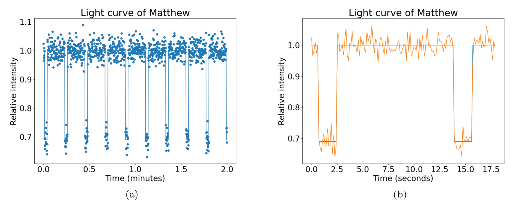
Both native Light curve of Matthew panels: (a) blue relative-intensity points against Time (minutes), (b) orange relative-intensity curve against Time (seconds); all axes, ticks, titles and panel labels. — Figure 1: Light Curves of Matthew

Although Matthew is too dim for David to achieve a reasonable SNR, as an observational master, David uses his knowledge of the dark arts to remove enough noise to do basic photometry experiments. Performing photometry on Matthew, David once again notices something interesting. Matthew’s light curve has periodic dips! Figure 1 shows plots of the light curve.

(f) David hypothesizes that these dips are due to trees being planted at regular intervals along the route, blocking some fraction of the sunlight incident on Matthew (you may assume that the trees are not directly over Matthew and so they do not block any of the light reflected off him).

(i) (5 points) How far apart are these trees planted?

(ii) (5 points) Estimate the width of each tree.

(iii) (8 points) By what factor does each tree reduce the incoming sunlight?

Отговори

Решение

Key-only statement variant (solution PDF page 15, part (f)(iii)): The key asks “What percentage of the incoming sunlight is blocked by the tree?” The question booklet instead asks “By what factor does each tree reduce the incoming sunlight?” Both formulations are preserved; the printed worked result is a percentage.

(a) There are two sources of luminosity emitted by Matthew: gray body radiation and reflected sunlight.

The gray body radiation is simply given by our modified Stefan-Boltzmann Law, which gives $(1-a)A\sigma T^4=409.2\ \mathrm W$ .

The contribution from reflected sunlight can be calculated by taking the flux from the Sun, multiplying by $1-a_\oplus$ to take into account the portion of sunlight reflected by the Earth’s atmosphere, and then multiplying by the albedo of Matthew and the area of Matthew. This gives

(1-a_\oplus)a\frac{L_\odot}{4\pi(1\ \mathrm{AU})^2}A=1114.5\ \mathrm W.

The total luminosity of Matthew is therefore $L=1524\ \mathrm W$ .

To get his apparent magnitude, we also need how far he is away from the telescope. We know that the telescope is in geostationary orbit, so we can calculate it’s orbital radius:

r=\sqrt{\frac{GM_\oplus}{\omega^3}}=4.22\times10^7\ \mathrm m

Note: here we used $\omega=2\pi/T_{\mathrm{sidereal}}$ . Solutions using $T=86\,400\ \mathrm s$ should also be accepted for full credit because the difference is very small.

To get the distance between Matthew and TESS, we simply subtract the radius of the Earth.

Finally, if we let $M$ and $m$ be the absolute and apparent magnitudes of Matthew, respectively, then we can use the equations

M-M_\odot=-2.5\log_{10}\left(\frac L{L_\odot}\right)\qquad\text{and}\qquad m-M=5\log_{10}\left(\frac{r-R_\oplus}{10\ \mathrm{pc}}\right)

We get that

m=M_\odot-2.5\log_{10}\left(\frac L{L_\odot}\right)+5\log_{10}\left(\frac{r-R_\oplus}{10\ \mathrm{pc}}\right)=\boxed{13.56}

(b) We can get the photon flux from Matthew by using

m-m_0=-2.5\log_{10}\left(\frac P{1\ \mathrm{e^-/s}}\right)

We get

P=10^{(m_0-m)/2.5}\ \mathrm{e^-/s}=10^{(20.44-13.56)/2.5}\ \mathrm{e^-/s}=563.7\ \mathrm{e^-/s}

Now the maximum SNR is obtained by the longest exposure possible before the pixel saturates. (We can prove this, but solutions that just state this intuition should be given full credit).

We will get an exposure time $t$ equal to

t=\frac{200\,000\ \mathrm{e^-}}P=\boxed{354.8\ \mathrm s}

We can plug this exposure time into the formula given to get the SNR:

\mathrm{SNR}=\frac{Pt}{\sqrt{Pt+Dt+N^2}}=\boxed{446.7}

(c) We can calculate the luminosity from the ground. First, we want the area of the ground that is captured by 1 pixel. To do this, we can use the plate scale formula to calculate the angular size of each pixel:

\theta=\frac yf=\frac{15\ \mu\mathrm m}{3.14\ \mathrm m}=4.78\times10^{-6}\ \mathrm{rad}

Multiplying this by the distance to ground, we get that the pixel is a square with side length

l=\theta(r-R_\oplus)=171\ \mathrm m\quad\Longrightarrow\quad A=l^2=2.93\times10^4\ \mathrm{m^2}

Now we can break up the luminosity from the ground into a reflected component an a graybody component. Similar to part (a), our graybody component is $(1-a_\oplus)\sigma AT^4=8.57\times10^6\ \mathrm W$ .

For the reflected component, we can simply take the flux from the Sun and multiply it by the area of the ground and the albedo of the ground:

a_\oplus\frac{L_\odot}{4\pi(1\ \mathrm{AU})^2}A=1.19\times10^7\ \mathrm W

Adding these together gives a total luminosity of $2.05\times10^7\ \mathrm W$ . Using the same formula in part (a), we get that

m=M_\odot-2.5\log_{10}\left(\frac L{L_\odot}\right)+5\log_{10}\left(\frac{r-R_\oplus}{10\ \mathrm{pc}}\right)=3.24

Now by the same logic as part (b), we get $P_b=10^{(m_0-m)/2.5}\mathrm{e^-/s}=7.56\times10^6\ \mathrm{e^-/s}$ .

Now all we need to do is recalculate the time:

t=\frac{200\,000\ \mathrm{e^-}}{P+P_b}=\boxed{0.0263\ \mathrm s}

and then plug this into a modified SNR formula:

\mathrm{SNR}=\frac{Pt}{\sqrt{Pt+P_bt+Dt+N_r^2}}=\boxed{0.0332}

(d) We calculated the angular size of each pixel in part (c). Now all we have to do is divide this by 45 seconds and convert to arcseconds per minute:

\omega=\frac\theta t=3.33\times10^{-7}\ \mathrm{rad/s}=\boxed{1.31\ \mathrm{arcsec/min}}

(e) For this part, we simply take the angular velocity in part (d) and multiply it by the distance from the satellite to the ground:

v=\frac{\theta\cdot(r-R_\oplus)}t=\boxed{3.80\ \mathrm{m/s}}

(f) Note: graders should be lenient about values read off the graphs.

(i) We can see in the first graph that 9 intervals happen in just under 2 minutes. Therefore, we can use a value of $\frac{120\ \mathrm s}9=13.33\ \mathrm s$ as the time between two trees (the actual value used to generate the graphs was 13.20 s).

Multiplying this value by the velocity in part (e), we get

l=13.2\ \mathrm s\cdot3.80\ \mathrm{m/s}=\boxed{50.2\ \mathrm m}

(ii) From the second graph, we can tell a dip lasts for approximately 3/4 of a x-axis tick, or 1.875 s (the actual value used to generate the graphs was 1.80 s).

Again, we simply need to multiply by the velocity in part (e) to get a tree width of

w=1.80\ \mathrm s\cdot3.80\ \mathrm{m/s}=\boxed{6.84\ \mathrm m}

(iii) From the second graph we can read a transit depth of approximately 0.3 (the actual value used to generate the graph was 0.31).

From part (a), we got that the luminosity of Matthew was 1524 W, with 409.2 W coming from graybody radiation and 1114.5 W coming from reflected sunlight.

We know that the tree blocked $0.31\cdot1524\ \mathrm W=472.3\ \mathrm W$ . Since we are told to assume that the tree only blocks sunlight and not any of his graybody radiation, the percent of incoming sunlight blocked is simply

\frac{472.3\ \mathrm W}{1114.5\ \mathrm W}=\boxed{42.4\%}

Source note: The orbital radius expression is printed as sqrt(GM/omega^3); no cubic root or different omega exponent is substituted. The first SNR evaluation has N^2 rather than the question’s N_r^2. The part(d) intermediate angular velocity conflicts with its given plate scale, elapsed time and final 1.31 arcsec/min. These printed expressions, results and all marking acceptance notes are retained. The solution’s own sunlight/graybody wording remains as printed.

Теми и трудност

Оценена трудност: 4/5.

Уреди и наблюдения · Светлина и астрономически измервания · Детектори и изображения · Звездни величини · Абсолютно черно тяло · Ъглов размер

Предпоставки: Гимназиална подготовка, Разширена олимпиадна подготовка

Оригинал в Архива: second_exam_2024.pdf · официални решения: second_exam_2024-solutions.pdf · допълнителни данни: physical-constants.pdf