Съдържание

USAAAO 2026, III кръг — Задача 1. Type II Supernova

Оригинал на условието (PDF)Съобщи за грешка

Всички материали от USAAAO 2026

2026 USAAAO Third Exam (Data Analysis + Observation) · 55 т.

Instructions (Please Read Carefully)

The test must be completed within 2 hours (120 minutes) and the maximum number of points is 230 points. The point breakdown per problem is as follows.

Problem	P1	P2	P3	P4	Total
Points	55	75	46	54	230

Please solve each problem on a blank piece of paper and mark the number of the problem at the top of the page. Some problems may require a designated answer sheet; these will be provided. The contestant's full name in capital letters should appear at the top of each solution page. If the contestant uses scratch papers, those should be labeled with the contestant's name as well and marked as “scratch paper” at the top of the page. Scratch paper will not be graded. Partial credit will be available given that correct and legible work was displayed in the solution.

This is a written exam. Contestants can only use a scientific calculator (non-programmable and non-graphing) for this exam. A table of physical constants will be provided. Discussing the problems with other people is strictly prohibited in any way until the end of the examination period on June 25, 2026. Receiving any external help during the exam is strictly prohibited. This means that the only allowed items are: a calculator, the provided table of constants, a pencil (or pen), an eraser, blank sheets of papers, and the exam. No books or notes are allowed during the exam. Students must be proctored during the entire duration of the exam.

This exam sheet and your answer sheets (including scratch papers) should be returned to your proctors once the exam ended. Your proctors should upload your answer sheets to the Google Form provided to them.

We acknowledge the following people for their contributions to this year's practical exam:

Ferdinand, Vincent Bian

After reading the instructions, please make sure to sign, affirming that:

All work on this exam has been completed by me.
I took this exam under the supervision of a proctor.
I did not receive any external help beyond the materials provided.
I will not discuss the contents of this exam with anyone until June 24, 2026.
Failure to follow these rules will result in disqualification from the exam.

Student Signature: ____________ Date: ____________

Условие

In April 2024, the Asteroid Terrestrial-impact Last Alert System (ATLAS) reported the emergence of a rapid brightening object in the constellation Hydra. Follow-up observations confirmed that the transient was a nearby Type II supernova located at $\sim 7.2$ Mpc, one of the closest supernovae of the decade. Due to its proximity, the supernova, named SN 2024ggi, has been well-characterized in multiple wavelengths. It was revealed that the expanding supernova shock was moving outward at a nearly constant velocity of 10,000 km/s. Prior to the explosion, the progenitor star had been losing mass through a slow stellar wind with a velocity of 20 km/s, creating a dense circumstellar medium (CSM) around the star.

When the rapidly expanding shock collides with this surrounding material, the gas is heated to temperatures of millions of kelvin and emits strongly in X-rays. As such, X-ray observations are the best tracer to constrain supernovae properties. X-ray observations in 2024 revealed the supernova's unabsorbed/intrinsic fluxes and emission measure $^{1}$ (EM) and can be summarized in the table below.

Table 1: Observed unabsorbed flux and emission measure of the supernova

Time since explosion (days)	Unabsorbed Flux (erg s $^{-1}$ cm $^{-2}$ )	EM (cm $^{-3}$ )
5.3	$7.11 \times 10^{-13}$	$2.75 \times 10^{62}$
10.9	$4.98 \times 10^{-13}$	$9.31 \times 10^{61}$
15.0	$2.54 \times 10^{-13}$	$6.08 \times 10^{61}$
16.2	$2.85 \times 10^{-13}$	$4.76 \times 10^{61}$
24.5	$1.66 \times 10^{-13}$	$3.76 \times 10^{61}$
34.8	$1.31 \times 10^{-13}$	$1.84 \times 10^{62}$
43.2	$1.02 \times 10^{-13}$	$1.07 \times 10^{62}$
55.0	$0.75 \times 10^{-13}$	$2.80 \times 10^{61}$
85.4	$0.55 \times 10^{-13}$	$2.16 \times 10^{61}$

In this problem, we are trying to find out the brightness decay rate of a supernova and calculate the mass-loss rate of the supernova progenitor through the shock interactions with the circumstellar medium (CSM). For this problem, please report the final answer using time in days and other parameters in cgs (centimeter-gram-seconds) units.

$^{1}$ Emission measure (EM), usually used in X-ray and Extreme Ultraviolet astronomy, is the number density of electron times the number density of ion integrated over volume of the region. In other words: $\mathrm{EM} = \int n_e n_I \, dV$ .

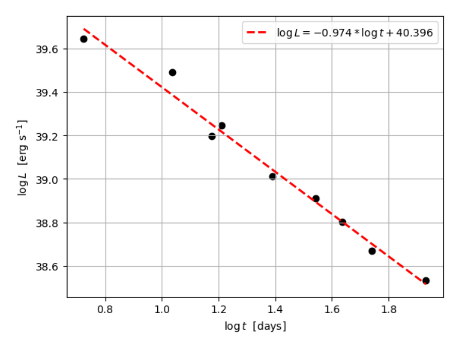
(a) Plot the luminosity vs time (in the provided grid paper). The luminosity vs time has a power-law relation, i.e. $L = At^{\alpha}$ , please estimate $A$ and $\alpha$ to get the relation and draw the relation in the plot too. Hint: it may be useful to draw a log-log plot. [20 т.]

(b) As the supernova explosion expands, the surrounding CSM of the supernova is being affected. Brethauer (2022) derived that the unshocked CSM density is expressed by:

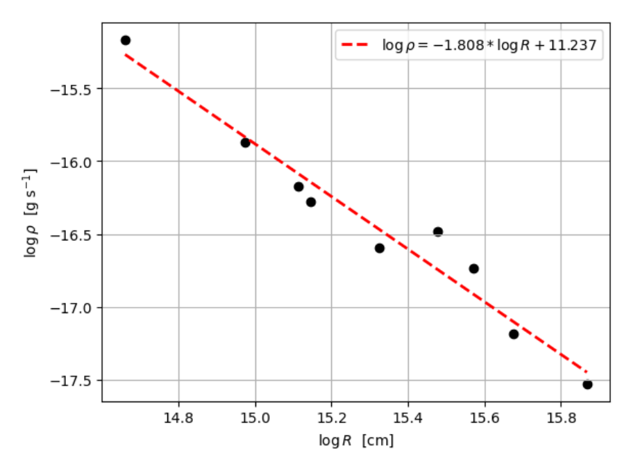
\rho_{\mathrm{CSM}} = \frac{m_p}{4}\sqrt{\frac{2 \times \mathrm{EM} \times \mu_e \times \mu_I}{V_{\mathrm{FS}}}}

where $m_p$ is the mass of proton, $\mu_e$ is the mean molecular weight per electron and can be assumed to be $\mu_e = 1.14$ , $\mu_I$ is the mean molecular weight per ion and can be assumed to be $\mu_I = 1.24$ , and $V_{\mathrm{FS}} \approx \frac{4}{3}\pi\left((1.2 \cdot R_{\mathrm{shock}})^3 - R_{\mathrm{shock}}^3\right)$ is the volume of the forward shock. Now, find the unshocked CSM densities and plot them as a function of shock radius (in the provided grid paper). The density vs radius also has a power-law relation, i.e. $\rho = Br^{\beta}$ , please estimate $B$ and $\beta$ to get the relation and draw the relation in the plot too. Hint: it may be useful to draw a log-log plot. [23 т.]

(c) Based on your previous results, please find the mass-loss rate and uncertainty of the supernova progenitor in $M_{\odot}$ /yr. (Hint: What is the relationship between density, radius, wind speed, and mass-loss rate? Disregard your fitting results in part b) [12 т.]

Отговори

Решение

Solution: This problem is about the supernova SN 2024ggi and inspired by one of my research projects (The data is from there too!). Please read it in https://doi.org/10.3847/1538-4357/ae4ec6 for more background information or if you are interested in learning more about core-collapse supernova!

General plot rubric for this question:

Using less than 70% of the total area for the graph	Deduct 20% of the marks for correct graph
Non-constant scale for axis	Deduct 20% of the marks for correct graph
Missing or incorrect labels or units in the axes	Deduct 20% of the marks for correct graph

(a) The luminosity is calculated from the observed unabsorbed flux using

L = 4\pi D^2 F,

where $D = 7.2$ Mpc $= 7.2 \times 10^6$ pc $= 2.22 \times 10^{25}$ cm. (3 points) Calculating the luminosity for each observation, we can get (5 points)

$t$ (days)	$\log_{10}(t)$	$F$ (erg s $^{-1}$ cm $^{-2}$ )	$L$ (erg s $^{-1}$ )	$\log_{10}(L)$
5.3	0.724	$7.11 \times 10^{-13}$	$4.41 \times 10^{39}$	39.644
10.9	1.037	$4.98 \times 10^{-13}$	$3.09 \times 10^{39}$	39.490
15.0	1.176	$2.54 \times 10^{-13}$	$1.58 \times 10^{39}$	39.199
16.2	1.210	$2.85 \times 10^{-13}$	$1.77 \times 10^{39}$	39.248
24.5	1.389	$1.66 \times 10^{-13}$	$1.03 \times 10^{39}$	39.013
34.8	1.542	$1.31 \times 10^{-13}$	$8.13 \times 10^{38}$	38.910
43.2	1.635	$1.02 \times 10^{-13}$	$6.33 \times 10^{38}$	38.801
55.0	1.740	$0.75 \times 10^{-13}$	$4.65 \times 10^{38}$	38.667
85.4	1.931	$0.55 \times 10^{-13}$	$3.41 \times 10^{38}$	38.533

Then, fit the luminosity decay rate with power law:

L = At^{\alpha} \quad \leftrightarrow \quad \log L = \alpha \log t + C

We get $\alpha \approx -0.974$ and $C = 40.396$ or in other words:

\log L = -0.974 \log t + 40.396

(5 points) The plot: (7 points)

Scatter plot of log L [erg s^-1] (vertical axis, 38.6 to 39.6) against log t [days] (horizontal axis, 0.8 to 1.8) with nine black data points and a red dashed fit line; legend: log L = −0.974 * log t + 40.396.

(b) The shock radius is

R_{\mathrm{shock}} = v_{\mathrm{shock}} t,

where $v_{\mathrm{shock}} = 10000\ \mathrm{km\ s^{-1}} = 1.0 \times 10^9\ \mathrm{cm\ s^{-1}}$ . (3 points) Using the fact that $\mathrm{EM} = \int n_e \cdot n_I \, dV$ , the unshocked CSM density is

\rho_{\mathrm{CSM}} = \frac{m_p}{4}\sqrt{\frac{2 \times \mathrm{EM} \times \mu_e \times \mu_I}{V_{\mathrm{FS}}}}

where $m_p = 1.67 \times 10^{-24}$ g, $\mu_e = 1.14$ , and $\mu_I = 1.24$ . Calculating the unshocked CSM density, we can get (7 points)

$t$ (days)	$R_{\mathrm{shock}}$ (cm)	$\log_{10}(R_{\mathrm{shock}})$	$\rho_{\mathrm{CSM}}$ (g cm $^{-3}$ )	$\log_{10}(\rho_{\mathrm{CSM}})$
5.3	$4.58 \times 10^{14}$	14.661	$6.81 \times 10^{-16}$	$-15.167$
10.9	$9.42 \times 10^{14}$	14.974	$1.34 \times 10^{-16}$	$-15.873$
15.0	$1.30 \times 10^{15}$	15.114	$6.73 \times 10^{-17}$	$-16.172$
16.2	$1.40 \times 10^{15}$	15.146	$5.30 \times 10^{-17}$	$-16.276$
24.5	$2.12 \times 10^{15}$	15.326	$2.54 \times 10^{-17}$	$-16.595$
34.8	$3.01 \times 10^{15}$	15.479	$3.31 \times 10^{-17}$	$-16.480$
43.2	$3.73 \times 10^{15}$	15.572	$1.83 \times 10^{-17}$	$-16.738$
55.0	$4.75 \times 10^{15}$	15.677	$6.50 \times 10^{-18}$	$-17.187$
85.4	$7.38 \times 10^{15}$	15.868	$2.95 \times 10^{-18}$	$-17.530$

Then, fit the density and shocked radius with a power law,

\rho_{\mathrm{CSM}} = BR_{\mathrm{sh}}^{\beta} \quad \leftrightarrow \quad \log \rho_{\mathrm{CSM}} = \beta \log R_{\mathrm{sh}} + K

We get $\beta \approx -1.808$ and $K = 11.237$ or in other words:

\log \rho_{\mathrm{CSM}} = -1.808 \log R_{\mathrm{sh}} + 11.237

(5 points) The plot: (8 points)

Scatter plot of log ρ (vertical axis, −17.5 to −15.5) against log R [cm] (horizontal axis, 14.8 to 15.8) with nine black data points and a red dashed fit line; legend: log ρ = −1.808 * log R + 11.237. The vertical axis label reads log ρ [g s^-1].

\rho_{\mathrm{CSM}} = \frac{\dot{M}}{4\pi R^2 v_{\mathrm{wind}}} \quad \leftrightarrow \quad \dot{M} = 4\pi R^2 \rho_{\mathrm{CSM}} v_{\mathrm{wind}}.

(3 points) This is why your $\beta$ value in part b should be near $-2$ . However, since our data was not perfect, we should disregard our fitting results from part b. Using $v_{\mathrm{wind}} = 20\ \mathrm{km\ s^{-1}} = 2 \times 10^6\ \mathrm{cm\ s^{-1}}$ , we can get the mass loss rate: (5 points)

$R_{\mathrm{shock}}$ (cm)	$\rho_{\mathrm{CSM}}$ (g cm $^{-3}$ )	$\dot{M}$ ( $M_{\odot}\,\mathrm{yr}^{-1}$ )
$4.58 \times 10^{14}$	$6.81 \times 10^{-16}$	$5.69 \times 10^{-5}$
$9.42 \times 10^{14}$	$1.34 \times 10^{-16}$	$4.75 \times 10^{-5}$
$1.30 \times 10^{15}$	$6.73 \times 10^{-17}$	$4.52 \times 10^{-5}$
$1.40 \times 10^{15}$	$5.30 \times 10^{-17}$	$4.15 \times 10^{-5}$
$2.12 \times 10^{15}$	$2.54 \times 10^{-17}$	$4.54 \times 10^{-5}$
$3.01 \times 10^{15}$	$3.31 \times 10^{-17}$	$1.20 \times 10^{-4}$
$3.73 \times 10^{15}$	$1.83 \times 10^{-17}$	$1.01 \times 10^{-4}$
$4.75 \times 10^{15}$	$6.50 \times 10^{-18}$	$5.86 \times 10^{-5}$
$7.38 \times 10^{15}$	$2.95 \times 10^{-18}$	$6.41 \times 10^{-5}$

and the mean value (2 points) and the uncertainty (i.e. standard deviation) (2 points) is

\boxed{\dot{M} \approx (6.4 \pm 2.6) \times 10^{-5}\ M_{\odot}\ \mathrm{yr}^{-1}.}

Using sample standard deviation is also okay, getting an error of $\sim 2.8 \times 10^{-5}\ M_{\odot}\ \mathrm{yr}^{-1}$

Оригинал в Архива: practical.pdf · официални решения: practical_solutions.pdf