Съдържание

Условие a. (8 т.)b.–f.Решение

USAPhO 2006, Полуфинал — B2

Оригинал на условието (PDF)Съобщи за грешка

Всички материали от USAPhO 2006

2006 Semi-Final Exam · 50 т.

2006 Semi-Final Exam — Instructions

AAPT / AIP — United States Physics Team 2006.

DO NOT OPEN THIS TEST UNTIL YOU ARE TOLD TO BEGIN

Work Part A first. You have 90 minutes to complete all four problems.
After you have completed Part A, you may take a break.
Then work Part B. You have 90 minutes to complete both problems.
Show all your work. Partial credit will be given.
Start each question on a new sheet of paper. Be sure to put your name in the upper right-hand corner of each page, along with the question number and the page number/total pages for this problem. For example: Doe, Jamie; A1 – 1/3.
A hand-held calculator may be used. Its memory must be cleared of data and programs. You may use only the basic functions found on a simple scientific calculator. Calculators may not be shared. Cell phones, PDA’s, or cameras may not be used during the exam or while the exam papers are present. You may not use any tables, books, or collections of formulas.
Questions with the same point value are not necessarily of the same difficulty.
Do not discuss the contents of this exam with anyone until after March 20th.
Good luck!

Possibly Useful Information – (Use for both part A and for part B)

Quantity	Value
Gravitational field at the Earth’s surface	$g=9.8$ N/kg
Newton’s gravitational constant	$G=6.67\times10^{-11}$ N·m $^2$ /kg $^2$
Coulomb’s constant	$k=1/4\pi\epsilon_0=8.99\times10^9$ N·m $^2$ /C $^2$
Biot-Savart constant	$k_m=\mu_0/4\pi=10^{-7}$ T·m/A
Speed of light in a vacuum	$c=3.00\times10^8$ m/s
Boltzmann’s constant	$k_B=1.38\times10^{-23}$ J/K
Avogadro’s number	$N_A=6.02\times10^{23}$ (mol) $^{-1}$
Ideal gas constant	$R=N_Ak_B=8.31$ J/(mol·K)
Stefan-Boltzmann constant	$\sigma=5.67\times10^{-8}$ J/(s·m $^2$ ·K $^4$ )
Elementary charge	$e=1.602\times10^{-19}$ C
1 electron volt	$1\text{ eV}=1.602\times10^{-19}$ J
Planck’s constant	$h=6.63\times10^{-34}\text{ J}\cdot\text{s}=4.14\times10^{-15}\text{ eV}\cdot\text{s}$
Electron mass	$m=9.109\times10^{-31}\text{ kg}=0.511\text{ MeV}/c^2$
Binomial expansion	$(1+x)^n\approx1+nx$ for $\lvert x\rvert\ll1$
Small angle approximations	$\sin\theta\approx\theta$ , $\cos\theta\approx1-\tfrac12\theta^2$

Условие

In this problem, we present a simple model of seasonal temperature variation. We ignore temperature and illumination changes between day and night, considering only daily average values. We also ignore all forms of heat transfer other than radiation, including any heat transfer between areas of the surface of the Earth. Finally, we ignore the effects of the atmosphere and clouds.

We therefore consider a patch of ground with heat capacity per unit area $c$ and emissivity $\epsilon$ , illuminated by light of varying intensity $I$ . The patch therefore has a varying temperature $T$ .

a. (8 т.)

Develop an equation relating $T$ , $\frac{dT}{dt}$ , $I$ , $c$ , $\epsilon$ , and the Stefan-Boltzmann constant $\sigma$ .

b.–f.

Figure 1 shows the yearly variation in average daily sunlight intensity on Earth for various latitudes. The variation is not sinusoidal, but for temperate latitudes, it may be approximated as a sinusoid. In particular, Figure 2 shows the variation in College Park, Maryland (at $39^\circ$ N latitude), together with a good sinusoidal approximation. Therefore, we assume that the intensity has the form $I=I_0+I_1\sin(\omega t)$ . If the annual variation in temperature is small compared to the absolute temperature, we will likewise have $T=T_0+T_1\sin(\omega t-\phi)$ , where by hypothesis $T_1\ll T_0$ .

Figure1: Relative daily sunlight intensity versus time in years for several latitudes.

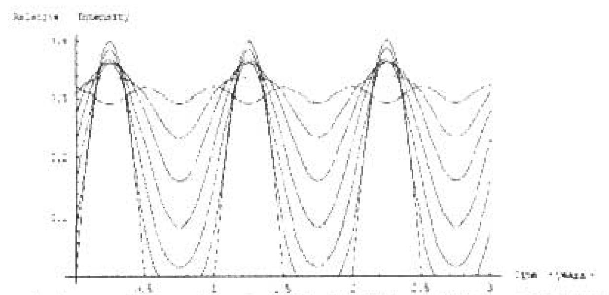
Figure 1: Average daily sun intensity on Earth ( $23.5^\circ$ axis tilt) for various latitudes. The vertical scale is normalized so that the intensity when the sun is overhead is 1.

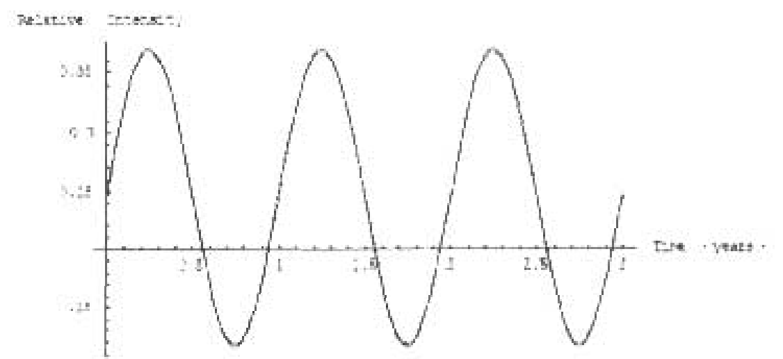
Figure2: College Park average daily intensity and sinusoidal fit.

Figure 2: Average daily sun intensity in College Park, with sinusoidal fit. The fit has equation $0.244-0.126\sin(2\pi t)$ .

b. Show that your previous result now implies an equation of the form

A+B\sin(\omega t-\phi)+C\cos(\omega t-\phi)=I_0+I_1\sin(\omega t)\qquad (1)

and provide the expressions for $A$ , $B$ , and $C$ in terms of $T_0$ , $T_1$ , $c$ , $\epsilon$ , $\sigma$ , and $\omega$ . [14 т.]

c. Using equation (1), find expressions for $A$ , $B$ , and $C$ in terms of $I_0$ , $I_1$ , and $\phi$ . [9 т.]

d. Combine your results to obtain a simple relationship between the relative amplitude of intensity fluctuations $I_1/I_0$ , the relative amplitude of temperature fluctuations $T_1/T_0$ , and the phase shift $\phi$ . [7 т.]

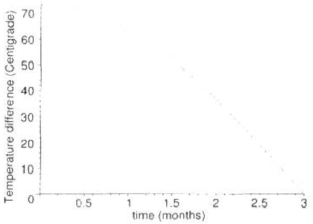
e. Plot on graph paper the predicted difference between summer and winter temperatures in Kelvin vs. the number of months between the summer solstice (day of maximum sunlight intensity) and the hottest day of the year. Use the values for $I_0$ and $I_1$ given for College Park in Figure 2, and assume a mean temperature of 283 K. Show work indicating the method of your calculations for the numbers plotted on the graph. [9 т.]

f. Actual temperature data for College Park is shown in Figure 3. Does the model provide a reasonable fit to the data? Briefly justify your answer. (The summer solstice occurs on June 21.)

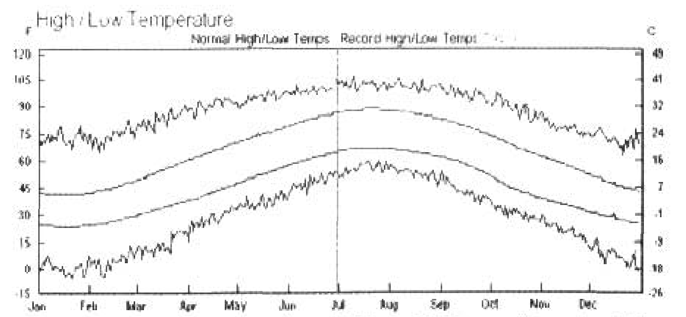
Figure3: BWI normal and record high/low temperatures throughout the year, Fahrenheit and Celsius scales.

Figure 3: Actual average temperature data at Baltimore-Washington International Airport. The vertical line is June 30. Source: Weather Underground, http://www.wunderground.com/. [3 т.]

Решение

Source note: the printed signs in (B2-15) and (B2-16) differ from the preceding and following lines; they are retained as printed. The question’s Figure2 caption prints a minus sign in its fitted sinusoid.

a. (8 т.)

The radiation power absorbed by the patch of area $a$ is

\epsilon aI,\qquad (B2-1)

while the power radiated from the patch is

\epsilon a\sigma T^4.\qquad (B2-2)

The imbalance causes a temperature change given by

ca\frac{dT}{dt}=\epsilon aI-\epsilon a\sigma T^4,\qquad (B2-3)

\frac c\epsilon\frac{dT}{dt}=I-\sigma T^4.\qquad (B2-4)

b. (14 т.)

We will need to do an expansion of $T^4$ .

T^4=T_0^4\left(1+\frac{T_1}{T_0}\sin(\omega t-\phi)\right)^4,\qquad (B2-5)

\approx T_0^4\left(1+4\frac{T_1}{T_0}\sin(\omega t-\phi)\right).\qquad (B2-6)

Insert this and the given expression for $I$ into Eq. B2-4,

\frac c\epsilon(T_1\omega\cos(\omega t-\phi))=\qquad (B2-7)

I_0+I_1\sin(\omega t)-\sigma T_0^4\left(1+4\frac{T_1}{T_0}\sin(\omega t-\phi)\right),\qquad (B2-8)

\sigma T_0^4+4\sigma T_0^3T_1\sin(\omega t-\phi)+\frac{c\omega T_1}{\epsilon}\cos(\omega t-\phi)=I_0+I_1\sin(\omega t).\qquad (B2-9)

Clearly, then,

A=\sigma T_0^4,\qquad (B2-10)

B=4\sigma T_0^3T_1,\qquad (B2-11)

C=\frac{c\omega T_1}{\epsilon}.\qquad (B2-12)

c. (9 т.)

The only way that it can work is if $A=I_0$ . Of course, one would expect the average intensity to be related to the average temperature in this way.

Expand the left hand sine and cosine terms according to the angle addition formulae:

\sin(\omega t-\phi)=-\cos\omega t\sin\phi+\sin\omega t\cos\phi,\qquad (B2-13)

\cos(\omega t-\phi)=\cos\omega t\cos\phi+\sin\omega t\sin\phi.\qquad (B2-14)

Substitute into Equation (1) from the question paper.

B(-\cos\omega t\sin\phi+\sin\omega t\cos\phi)+C(\cos\omega t\cos\phi-\sin\omega t\sin\phi)=I_1\sin\omega t.\qquad (B2-15)

This, after collecting terms, yields

(-B\sin\phi-C\cos\phi)\cos\omega t+(B\cos\phi+C\sin\phi)\sin\omega t=I_1\sin\omega t.\qquad (B2-16)

The cosine term must vanish, and this only happens if

-B\sin\phi+C\cos\phi=0,\qquad (B2-17)

leaving the sine term, so

B\cos\phi+C\sin\phi=I_1.\qquad (B2-18)

Combining,

B\cos\phi+B\frac{\sin\phi}{\cos\phi}\sin\phi=I_1,\qquad (B2-19)

B=I_1\cos\phi,\qquad (B2-20)

and then

C=B\frac{\sin\phi}{\cos\phi}=I_1\sin\phi.\qquad (B2-21)

d. (7 т.)

Evaluate $B/A$ .

\frac BA=\frac{I_1}{I_0}\cos\phi,\qquad (B2-22)

and

\frac BA=\frac{4\sigma T_0^3T_1}{\sigma T_0^4}=4\frac{T_1}{T_0},\qquad (B2-23)

we have

\frac{I_1}{I_0}\cos\phi=4\frac{T_1}{T_0}.\qquad (B2-24)

Since $I_1/I_0=0.126/0.244=0.516$ we ought be concerned that $T_1/T_0$ might not be a sufficiently small quantity for this approximation!

e. (9 т.)

Since the temperature difference is twice the oscillation amplitude,

\Delta T=2T_1,\qquad (B2-25)

so we are interested in graphing

\Delta T=\frac{T_0}{2}\frac{I_1}{I_0}\cos\phi,\qquad (B2-26)

=(73.1\text{ K})\cos\left(t\frac\pi{6\text{ month}}\right).\qquad (B2-27)

Official predicted temperature difference (Centigrade) versus time lag in months, from0 to3months.

f. (3 т.)

According to the data on the question paper the peak temperature happens about one month after the solstice. The predicted summer/winter temperature difference would then be about $62\,\mathrm{C}^\circ$ , which is about 2.5 times that seen in the average temperature data for BWI.

Оригинал в Архива: Semifinal 2006.pdf · официални решения: Semifinal 2006 Solutions.pdf