Съдържание

USAPhO 2021, Финален кръг · подбор на отбора — Задача 2. The Dark Forest

Оригинал на условието (PDF)Съобщи за грешка

Всички материали от USAPhO 2021

2021 USAPhO+ — Traveling Team Selection Exam · 8 май 2021 г.

Information About The 2021 USAPhO+

The 2021 USAPhO+ is a 5-hour exam taking place on Saturday, May 8 from noon to 5 PM, Eastern time.
The exam is hosted by AAPT on the platform provided by Art of Problem Solving. It will be proctored by the US Physics Team coaches via Zoom.
Before you start the exam, make sure you are provided with blank paper, both for your answers and scratch work, writing utensils, graph paper and a ruler, a hand-held scientific calculator with memory and programs erased, and a computer for you to log into the USAPhO+ testing page.
At the end of the exam, you have 20 minutes to upload solutions to all of the problems for that part. For each problem, scan or photograph each page of your solution, combine them into a single PDF file, and upload them on the testing platform.
USAPhO+ graders are not responsible for missing pages or illegible handwriting. No late submissions will be accepted.

Congratulations again on your qualification for the USAPhO+. We wish you the best of luck on the challenging problems to follow.

We acknowledge the following people for their contributions to this year’s exam (in alphabetical order):

JiaJia Dong, Mark Eichenlaub, Abijith Krishnan, Kye W. Shi, Brian Skinner, Mike Winer, and Kevin Zhou.

Условие

Dark matter could be made of hypothetical, extremely light particles called axions. Because individual axions are so light, experiments do not search for individual axions, but rather for the classical axion field formed by a large collection of axions, which oscillates as

a(t) = a_0\sin(\omega t).

This is analogous to how a large collection of photons can form a classical electromagnetic field. In the presence of a magnetic field $\mathbf{B}$ and an axion field $a$ , the axion field produces an effective current

\mathbf{J} = g\dot{a}\mathbf{B}

where we define $\dot{a} = da/dt$ . The effective current produces electromagnetic fields in exactly the same way as ordinary current, though it does not come from the motion of actual charges. Experiments can search for axion dark matter using systems which are resonantly driven by this current.

You may use fundamental constants in your answers, such as

\begin{aligned} c &= 3.00\times10^8\,\mathrm{m/s} & \hbar &= 1.055\times10^{-34}\,\mathrm{J\cdot s} & e &= 1.602\times10^{-19}\,\mathrm{C} \\ G &= 6.67\times10^{-11}\,\mathrm{N\cdot m^2/kg^2} & \mu_0 &= 4\pi\times10^{-7}\,\mathrm{N/A^2} & k_B &= 1.38\times10^{-23}\,\mathrm{J/K}. \end{aligned}

You do not have to provide numeric answers unless asked. When asked to “estimate”, you may drop constants of order one. The numeric values provided below are from standard references where $\hbar$ , $c$ , $\mu_0$ , and $\epsilon_0$ are set to one; to get correct numeric results, you must restore these factors yourself.

1

First, we will describe some physical properties of the axion field.

(a) Consider a single axion at rest, with mass $m$ . Find its associated angular frequency $\omega$ . This will be the angular frequency of the corresponding classical field, when there are many axions.

(b) Suppose dark matter is distributed spherically symmetrically in the galaxy with uniform density $\rho$ . The solar system is a distance $r$ from the center of the galaxy and orbits around it with period $T$ . Neglecting everything besides dark matter, find the dark matter density $\rho$ .

(c) The energy density of the axion field is $m^2a_0^2/(2\hbar^3c)$ . Find the axion field amplitude $a_0$ .

(d) The radius and period of the Sun’s orbit, as well as a typical axion mass, are

r = 2.5\times10^{20}\ \mathrm{m},\quad T = 7.1\times10^{15}\ \mathrm{s},\quad m = 1.0\times10^{-9}\ \mathrm{eV}.

Numerically compute the axion field amplitude $a_0$ .

(e) In this problem, we treat the axion field as spatially uniform within a terrestrial laboratory. To verify that this assumption is reasonable, numerically estimate the axion field’s wavelength $\lambda$ , assuming the axions have the same galactic speed as the Sun.

(f) In part (a), you found $\omega$ by neglecting the axion’s speed. In reality, the axion’s finite speed changes the frequency to $\omega + \Delta\omega$ , in a frame at rest with respect to the galactic center. Numerically estimate $\Delta\omega/\omega$ to show that it is reasonable to neglect this effect.

2

The ABRACADABRA $^1$ experiment, currently taking data at MIT, is a toroidal solenoid with inner and outer radius $R_{\mathrm{in}}$ and $R_{\mathrm{out}}$ and height $h$ . You may assume $h \gg R_{\mathrm{out}}$ for simplicity. A superconducting wire carrying current $I$ wraps $N$ times around the toroid, where $N$ is high enough to neglect the discreteness of the wires. A circular pickup loop with radius slightly less than $R_{\mathrm{in}}$ is placed at the center of the toroid.

Now, we will find the axion signal generated in the ABRACADABRA apparatus.

$^1$ aka, A Broadband/Resonant Approach to Cosmic Axion Detection with an Amplifying B-field Ring Apparatus.

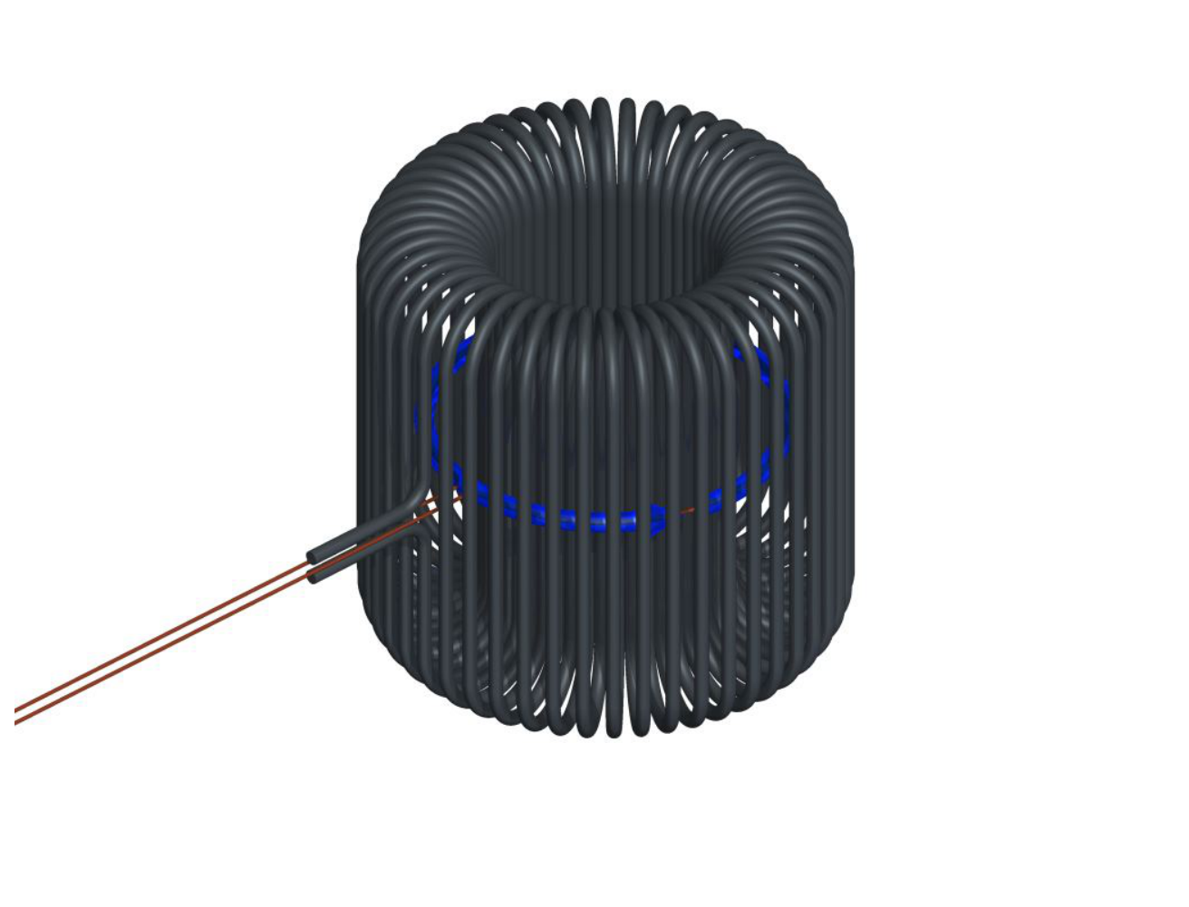
Rendered 3D view of the ABRACADABRA toroidal magnet: a tall toroid densely wound with dark superconducting wire, a blue circular pickup loop visible inside at the center, and a pair of copper leads running out to the lower left.

(a) Find the magnetic field $\mathbf{B}(\mathbf{r})$ inside the toroid due to the superconducting current.

(b) The superconducting wires lose their superconductivity when exposed to a magnetic field greater than $B_{\mathrm{max}}$ . Find the maximum possible current $I_{\mathrm{max}}$ that can be used, and assume this current is used in later parts.

(c) Assuming that $\omega$ is small, find the magnetic flux $\Phi_B(t)$ through the pickup loop due to the axion field in terms of $a_0$ , $g$ , $\omega$ , $B_{\mathrm{max}}$ , and the dimensions of the apparatus. (You may ignore any currents induced on the surfaces of the superconducting wires. Accounting for them makes the problem much harder, but does not substantially affect the final result.)

(d) If $\omega$ is too large, the result above breaks down due to radiation effects. Estimate the frequency $\omega_c$ where this happens.

(e) Using the design values

R_{\mathrm{in}} = 0.5\ \mathrm{m},\quad R_{\mathrm{out}} = 1.0\ \mathrm{m},\quad h = 2.0\ \mathrm{m}

estimate the numerical value of $\omega/\omega_c$ .

(f) Let $\Phi_0$ be the amplitude of the time-varying axion flux. Using the typical values

B_{\mathrm{max}} = 5.0\ \mathrm{T},\quad g = 1.0\times10^{-16}\ \mathrm{GeV^{-1}}

and your previous results, compute the numerical value of $\Phi_0$ .

3

The pickup loop has inductance $L$ and is attached to a capacitor, forming a circuit with resonant frequency equal to the axion frequency $\omega$ . The circuit also has a small internal resistance $R$ in series, and is at temperature $T$ . The axion signal can be detected by monitoring the current in the circuit. The main source of noise is thermal noise, which causes fluctuations in the current.

We will now estimate the sensitivity of ABRACADABRA to axions.

(a) The axion produces a current which oscillates sinusoidally. Find the signal current amplitude $I_s$ in terms of $\omega$ , $\Phi_0$ , and the circuit parameters.

(b) Find the average value of the current squared $\langle I^2\rangle$ in the circuit due to thermal noise.

(c) At any moment in time, the noise current is oscillating sinusoidally with typical amplitude $I_n = \sqrt{\langle I^2\rangle}$ , which is much larger than $I_s$ . However, the phase of the noise current also fluctuates randomly, so that after a typical time $t_c$ , its phase will be roughly independent of the phase it had before. Find an estimate for $t_c$ in terms of $\omega$ and the circuit parameters. (Hint: at any given moment, the thermal noise current is simultaneously being produced by the random motion of electrons in the circuit, and damped by the resistor.)

(d) Suppose the experiment runs for a total time $t_e \gg t_c$ . Roughly estimate the average amplitude of the noise current over this period of time.

(e) The axion is detectable if the signal current amplitude is larger than the averaged noise current amplitude, and the circuit parameters are

L = 1\ \mathrm{mH},\quad R = 10\ \mathrm{m\Omega},\quad T = 0.1\ \mathrm{K}.

Roughly numerically estimate the time needed to potentially detect the axion. (Hint: if your answer seems strange, note that in reality, the axion’s phase also fluctuates over time, because of the effect of part 1(f). In addition, we don’t know $\omega$ ahead of time, so the experiment needs to be run many times. We ignored these effects here to keep things simple.)

Отговори

Решение

1

(a) The axion is a quantum particle and satisfies the de Broglie relation $E = \hbar\omega$ , and its energy comes from its rest mass, $E = mc^2$ . Thus,

\omega = \frac{mc^2}{\hbar}.

(b) Setting the centripetal acceleration equal to the gravitational acceleration,

r\omega^2 = \frac{GM}{r^2},\quad M = \frac{4}{3}\pi r^3\rho.

Solving for $\rho$ , we find

\rho = \frac{3\pi}{GT^2}.

(c) The dark matter density comes from the mass-energy of the axion field, so

\rho c^2 = \frac{m^2a_0^2}{2\hbar^3c},\quad a_0 = \sqrt{\frac{2\rho\hbar^3c^3}{m^2}}.

(d) Plugging in numbers and noting that the provided value of the axion mass is really its energy (and hence dividing it by $c^2$ ) gives the value

a_0 = 2.36\times10^{-4}\,\mathrm{kg\,m^3/s^3}.

(e) The axion speed is

v = \frac{2\pi r}{T} = 2\times10^5\,\mathrm{m/s}.

Using the de Broglie relation again,

\lambda = \frac{h}{p} = \frac{h}{mv} \sim 10^6\,\mathrm{m}.

As expected, this is much larger than the apparatus considered below. (Note: a common mistake was to write $v = f\lambda$ , but this is only true for waves which travel at a constant speed, such as light. To see the problem, note that if you apply the de Broglie relations, this equation becomes $v = E/p$ . That’s true for photons, where $E = pc$ , but certainly not true for massive particles. Some students also tried the Compton wavelength $\lambda = h/mc$ , but this is a different quantity, namely the wavelength of a photon if it had the same energy as an axion at rest.)

(f) Because $E = \hbar\omega$ , we need to see how the energy is changed. We have

\frac{\Delta E}{E} \approx \frac{mv^2/2}{mc^2} = \frac{v^2}{2c^2}

where we used the fact that $v$ , computed above, is nonrelativistic. We thus find

\frac{\Delta\omega}{\omega} \sim 3\times10^{-7}

which is small as expected. (Note that the usual Doppler shift formula would not work here, and trying to use it would get the wrong answer. The Doppler shift formula applies to particles with constant speed, which satisfy $\omega = vk$ . The axion is massive; when at rest, it has $\omega \neq 0$ and $k = 0$ . However, you could also get the answer by Lorentz transforming the four-vector $(\omega, \mathbf{k})$ .)

2

(a) Using Ampere’s law,

\mathbf{B} = \frac{\mu_0NI}{2\pi r}\,\hat{\theta}.

(b) The maximum field is at $r = R_{\mathrm{in}}$ , so

B_{\mathrm{max}} = \frac{\mu_0NI_{\mathrm{max}}}{2\pi R_{\mathrm{in}}},\quad I_{\mathrm{max}} = \frac{2\pi R_{\mathrm{in}}B_{\mathrm{max}}}{\mu_0N}.

(c) The effective current is

\mathbf{J} = g\dot{a}\mathbf{B} = ga_0B_{\mathrm{max}}\frac{R_{\mathrm{in}}}{r}\omega\cos(\omega t)\hat{\theta}.

The resulting field is like that of an array of concentric solenoids, where we may neglect fringe fields because $h \gg R_{\mathrm{out}}$ . Therefore, the axion-produced field $\mathbf{B}_{\mathrm{ax}}$ inside the pickup loop is uniform. For simplicity, we define

J_0 = ga_0B_{\mathrm{max}}\omega.

Then using Ampere’s law, we have

B_{\mathrm{ax}} = \mu_0J_0\cos(\omega t)\int\frac{R_{\mathrm{in}}}{r}\,dr = \mu_0J_0R_{\mathrm{in}}\log\bigl(R_{\mathrm{out}}/R_{\mathrm{in}}\bigr)\cos(\omega t).

The magnetic flux is then

\Phi_B = \pi R_{\mathrm{in}}^2B_{\mathrm{ax}} = \pi\mu_0J_0R_{\mathrm{in}}^3\log\bigl(R_{\mathrm{out}}/R_{\mathrm{in}}\bigr)\cos(\omega t).

(d) In the calculations above, we have assumed that the fields are quasistatic, neglecting the radiation propagation time. This approximation breaks down when

\omega_c \sim \frac{c}{R_{\mathrm{in}}}

past which the flux will be diminished. Since this calculation is approximate, the answers $c/R_{\mathrm{out}}$ or $c/h$ are also acceptable.

(e) Plugging numbers in, we find

\omega_c \sim 6.0\times10^8\,\mathrm{s^{-1}},\quad \omega \sim 1.5\times10^6\,\mathrm{s^{-1}}.

Then we have

\omega/\omega_c \sim 0.0025

which is small as expected. Any answer within an order of magnitude is acceptable.

(f) First, we have to restore the dimensions of $g$ . Notice that since current $g\dot{a}B$ has the same units as displacement current $\epsilon_0\dot{E}$ , the quantities $ga$ and $(E/B)\epsilon_0$ must have the same dimensions, and furthermore $E/B$ has dimensions of speed.

Now, in 1(c) we found that $a$ has dimensions of energy times velocity, while the value of $g$ given here has dimensions of inverse energy. Thus, the combination $ga$ only has dimensions of speed, which means a factor of $\epsilon_0$ was left out. In other words, if we denote the value given above as $g'$ , the true value of $g$ is $\epsilon_0g'$ .

To avoid mistakes, it’s best to group terms in the long expression for $\Phi_0$ , so that each piece has simple units and a reasonable magnitude. We have

\Phi_0 = (\pi R_{\mathrm{in}}^2B_0)\,\log\left(\frac{R_{\mathrm{out}}}{R_{\mathrm{in}}}\right)\,R_{\mathrm{in}}\,\mu_0\epsilon_0g'a_0\omega

and using $c^2 = 1/\mu_0\epsilon_0$ gives

\begin{aligned} \Phi_0 &= (\pi R_{\mathrm{in}}^2B_0)\,\log\left(\frac{R_{\mathrm{out}}}{R_{\mathrm{in}}}\right)\,\frac{\omega R_{\mathrm{in}}}{c}\,\frac{g'a_0}{c} \\ &= (3.9\,\mathrm{Wb})(0.693)(0.0025)(4.91\times10^{-19}) \\ &= 3.3\times10^{-21}\,\mathrm{Wb}. \end{aligned}

3

(a) Since the axion is at the resonant frequency, the impedance of the circuit is approximately $R$ . Therefore the current is

I = \frac{\mathcal{E}}{R} = -\frac{1}{R}\frac{d\Phi_B}{dt}.

The amplitude is

I_s = \frac{\omega\Phi_0}{R}.

(b) The energy stored in the inductor is $LI^2/2$ . By the equipartition theorem, the average energy stored in any such quadratic degree of freedom is $k_BT/2$ , so

\langle I^2\rangle = \frac{k_BT}{L}.

This effect is also called Johnson noise.

(c) The noise current that exists in the circuit at any given moment, by definition, came from the thermal motion of electrons in the circuit up to a time $t_c$ ago. Therefore, $t_c$ is roughly the characteristic time for decay of current in the circuit. There are many ways to calculate this, but a simple way is to note that

t_c \sim \frac{Q}{\omega},\quad Q = \frac{\omega L}{R}

where $Q$ is the quality factor. Thus,

t_c \sim \frac{L}{R}.

(d) Uncertainty goes down by $\sqrt{n}$ when averaging $n$ independent trials. Here we have $n = t_e/t_c$ , so

\bar{I}_n = I_n\sqrt{\frac{t_c}{t_e}}.

(e) By setting $I_s = \bar{I}_n$ and solving for $t_e$ , we find

t_e \sim \frac{k_BTR}{\omega^2\Phi_0^2} = 550\,\mathrm{s}.

In reality, you would need to repeat this experiment millions of times to scan a sufficient range of $\omega$ , and the time in each step would be longer, because after some point the average axion signal also starts going down as $1/\sqrt{n}$ .

Оригинал в Архива: 2021-USAPhO_plus.pdf · официални решения: 2021-USAPhO_plus_Solutions_v2.pdf