Съдържание

WoPhO 2012, Теория — Задача 3. Modeling Reservoir Depletion

Оригинал на условието (PDF)Съобщи за грешка

Всички материали от WoPhO 2012

Theoretical 2: Physics of the Oil and Gas Production

Условие

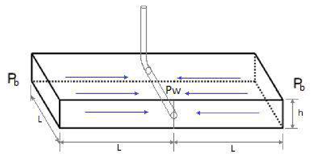
In this part the depletion process will be analyzed for the reservoir shown in Figure 8. The well has a horizontal part, therefore, the fluid flow in the reservoir is linear ( $h \ll L$ ).

A flat rectangular reservoir of height h, width L and length 2L (two halves of length L) with a well descending into its center, where the pressure is P_w; pressure P_b at both end faces; blue arrows show flow from both ends towards the well. — Figure 8: System used for modeling reservoir depletion

This time, pressure at the bottom of the well $P_w$ is constant (hydrostatic column of oil). However, the pressure at the boundary $P_b(t)$ is changing with time, as well as the oil production rate $q(t)$ . In this model the flow rate of the fluid is given by:

q = -2\varphi L^2 c_r h\frac{d\bar{P}}{dt}\ ,\qquad (5)

where $c_r$ is the compressibility of the rock, and the average pressure inside the reservoir $\bar{P}$ is approximated by:

\bar{P} \approx \frac{P_b + P_w}{2}.\qquad (6)

(a) Derive an explicit expression for $q(t)$ in terms of $k, \mu, c_r, \varphi$ and reservoir dimensions, if the initial flow rate is $q_0$ . [1,2 т.]

(b) For the system described in this section, determine the time needed to deplete the oil reservoir by a half. [1 т.]

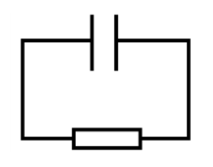
(c) Historically, first attempts to predict reservoir performance were made by doing analogies to electric circuits. Draw a simple electric circuit, which is analogous to the system described in Part 3. [0,5 т.]

(d) The reason why gas reservoirs cannot be modeled with the circuit as in 3.c, is that gas is highly compressible, with a compressibility being strongly dependent on the applied pressure. Compressibility is defined as:

c = -\frac{1}{V}\left(\frac{dV}{dP}\right)_T\ ,\qquad (7)

where $V$ is initial volume of the examined sample, $dV$ is isothermal volume change, when additional pressure $dP$ is applied.

Assuming natural gas as ideal, derive its compressibility $c_g$ as function of pressure $P$ . [0,3 т.]

Отговори

Решение

3.1

q = \frac{dV_{fluid}}{dt} = \frac{d(\varphi V_{res})}{dt} = \varphi V_{res}\left(\frac{1}{V_{res}}\frac{dV_{res}}{d\bar{p}}\right)\frac{d\bar{p}}{dt} = -2\varphi L^2 hc_r\frac{d\bar{p}}{dt}

\boxed{\alpha = -2\varphi L^2 hc_r}\qquad (3.1.1)

3.2 Applying Darcy’s law:

q = 2\frac{k}{\mu}Lh\frac{P_b - P_w}{L} = -2\varphi L^2 hc_r\frac{d\bar{p}}{dt}\qquad (3.2.1)

Average pressure can be estimated as:

\bar{p} \approx \frac{P_b + P_w}{2}\qquad (3.2.2)

Considering that $P_w$ is constant:

d\bar{p} \approx \frac{1}{2}dP_b\qquad (3.2.3)

Solving Eq.(3.2.3) and (3.2.1)

\int_{P_b(0)}^{P_b(t)}\frac{dP_b}{P_b - P_w} = -\frac{2k}{\mu L^2 c_r\varphi}\int_0^{t} dt

ln\left(\frac{P_b(t) - P_w}{P_b(t) - P_w}\right) = -\frac{2k}{\mu L^2 c_r\varphi}t

Using definition of the flow rate from Eq. (3.2.1)

ln\left(\frac{q(t)}{q_0}\right) = -\frac{2k}{\mu L^2 c_r\varphi}t

\boxed{q(t) = q_o exp\left(-\frac{2k}{\mu L^2 c_r\varphi}t\right)}\qquad (3.2.4)

3.3

V_{produced} = \int_o^T q(t)dt\qquad (3.3.1)

Using Eq. (3.2.4)

V_{produced} = -\frac{\mu L^2 c_r\varphi}{2k}q_o exp\left(-\frac{2k}{\mu L^2 c_r\varphi}t\right)\Big|_o^T = \frac{\mu L^2 c_r\varphi}{2k}q_o\left[1 - exp\left(-\frac{2k}{\mu L^2 c_r\varphi}T\right)\right]\qquad (3.3.2)

From the problem statement, volume of oil produced is a half of the initial reserves:

V_{produced} = \frac{1}{2}V_{res}\varphi = \frac{1}{2}(2L^2 h)\varphi\qquad (3.3.3)

Thus

\boxed{T = \frac{\mu L^2 c_r\varphi}{2k}ln\left(\frac{1}{1 - \frac{2kh}{\mu c_r q_0}}\right)}\qquad (3.3.4)

Equation (3.3.4) gives rather bad results for real data, because the fluid flow model was very rough, nevertheless order of the magnitude usually is very close to the results from numerical simulations.

3.4 Equation for the flow rate $\boldsymbol{q(t)}$ derived in the part 3.2 is an exponential decline. Similar equation could be obtained for the circuit with a capacitor and a resistor. There a flow rate is analogous to the charge at the capacitor plate and term with compressibility is analogous to the resistor.

A simple closed circuit consisting of a capacitor (top) and a resistor (bottom) connected in a loop.

3.5 Ideal gas law:

V = \frac{\vartheta RT}{P}\qquad (3.5.1)

Differentiating Eq. (3.5.1)

\left(\frac{dV}{dP}\right)_T = -\frac{1}{p^2}\vartheta RT\qquad (3.5.2)

Using definition of the compressibility and Eq. (3.5.2) results in

\boxed{c_g = -\frac{1}{V}\left(\frac{dV}{dP}\right)_T = \frac{1}{p}}\qquad (3.5.3)

As it is seen with higher pressure gas behaves more like a fluid, with negligible compressibility. However during production, when pressure drops significantly, gas production deviates from exponential decline.

Оригинал в Архива: WoPhO_2012_Q12.pdf · официални решения: WoPhO_2012_S12.pdf