EuPhO 2020, Експеримент — Задача 1. Hidden Charge
EuPhO-2020 Online. Experimental Problems. Language: English
Условие
1.1 Introduction
An unknown point charge is fixed in a region of space. Electrons launched parallel to the axis far from the charge will scatter electrostatically off of the fixed charge and strike a detecting screen. It is possible learn about the details of the hidden charge by varying the initial kinetic energy as well as the initial and coordinates of the electron beam and measuring the final coordinates and of where an electron strikes a finite flat screen perpendicular to the axis and located at .
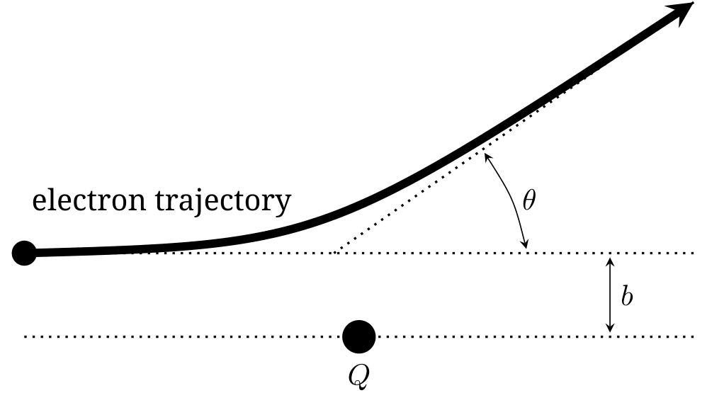
It is useful to know the Rutherford scattering formula,
where is the impact parameter, is the energy of the electron, is the charge of the electron, , and is the scattering angle. The impact parameter is defined as the closest approach of the electron to the target, assuming that the electron were unaffected by the target and hence would move in a straight line; the scattering angle is angle between the original velocity vector of the electron far from the target and the final velocity vector of the electron far from the target after scattering.
1.2 Task
The task is to determine the position and also the magnitude and sign of the fixed charge , as precisely as possible. You should provide rough, order of magnitude error estimates on these results. There is Gaussian error associated with initial beam location that is on the order of mm.
As with all experiments, you must provide clearly labelled tables of data, clearly labelled graphs, and sufficient formulae derivations to make it clear what you have measured, and how you are deriving your results.
1.3 Program Interface
The program asks for an accelerating voltage with the prompt
Beam accelerating voltage in V:
Enter a number between 1 and 10000, and press return. The program then asks for the initial launch coordinates, starting with , with the prompt
x-coordinate of the electron beam in cm:
Enter a number between -20 and 20 and then press return. Finally, the program asks for , with the prompt
y-coordinate of the electron beam in cm:
Enter a number between -20 and 20 and then press return. If you enter an invalid number for any of these three, the program will prompt you with
Invalid entry.
and will then prompt you for the value again, reminding you of the allowed limits.
After the three numbers have been entered, the program will output
Electron beam fired with parameters (x, y, V) =
and it will restate your entered values, and then
Electron detected at (x, y) =
and give the screen location of the detected electron. However, if the electron misses the finite size screen, you will be told
Electron not detected...
The program then repeats, allowing you to enter in a new set of initial coordinates.
Отговори
xQ ≈ 5.4 cm, yQ ≈ −2.6 cm, |zQ| ≈ 11.5 cm, Q ≈ −86 pC (|zQ| ≈ 9.9 pCm)
Reference values taken from the official grading scheme (parts 2 and 5).
Решение
1.1 Finding and
The first step is to locate the and coordinates of the test charge. Two approaches are illustrated here.
1.1.1 Method 1
Select any initial launch point, and keep it fixed. is a good choice. Vary the accelerating voltage in order to obtain several screen hits; plot these on a graph. Draw a line through the points, extended in both directions. The target charge must lie on this line.
Repeat with a different launch point. is a good choice. The two lines will intersect, this is likely the location of the target charge.
Select a third launch point, one that would be located approximately perpendicular to either of the first two lines. is a good choice. All three lines should intersect at a single point; that’s the location of the target charge,
1.1.2 Method 2
This method is much less accurate. Select a fixed value for , and vary . Observe . There will be a value of such that is almost the same, while on either side of it, will shift away from . This special value such that is the location . Repeat the process with a fixed and a varying . Not that this technique won’t work if the target charge is outside the bounds of the screen!
A student using this method cannot get full marks for the problem.
1.2 Determining and
Focus on the Rutherford equation. It is convenient to write it in the form
One choice is to try and keep fixed, and vary and . The other choice is to keep fixed and small, and vary . Each approach has benefits and drawbacks.
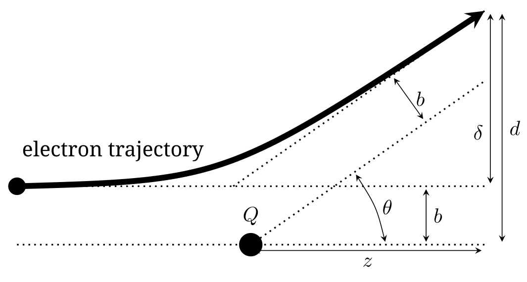
The Rutherford scattering equation diagram can also be drawn as below
1.2.1 Method 1: keep fixed
The screen distance is given by the relation
This is only strictly true if the electron has reached the scattered asymptote, otherwise, the measured value of will be larger than the true value.
For a fixed value of , which will happen if the product is kept constant, graph vertically against horizontally. The slope of the graph will yield the value of , the intercept will yield . The sign of is unimportant, as it was implied that it is behind the screen. Return to Rutherford’s equation to find .
One can improve the results by selecting values of that are small, as this forces the electron to be closer to the scattered asymptote.
Method 1A: focus on
One might think that it is easier to focus on the quantity , as it is directly measurable. The problem is that the intercept between the two asymptotes of the trajectory is not a distance from the screen, it is farther by an amount . Neglecting this correction will lead to from which the student can only find the product .
Including the correction yields a really ugly looking expression
Most efforts to reduce this expression will return the student to some equivalent of the previous paragraph, with only a value of obtainable.
1.2.2 Method 2: keep fixed and small
A second approach is to use the twice angle formula for the tangent:
Let , and then combining with the Rutherford equation,
where . If is small compared to , then . Combining, one gets the linear equation
Plotting vertically against horizontally ought yield a straight line with a slope and an intercept . The challenge here is the Gaussian error in the initial beam location; as gets smaller that relative error becomes more significant. If there were no initial beam spread, then this approach would be exact in the limit .
Method 2A: focus on
As before, this approach has the disadvantage that the intercept point of the trajectory asymptotes is a function of and . Neglecting this error, a student could graph vertically against horizontally. The student has gained some in that the error of has been removed from the expression for , but an error of has been added to the expression for . In this case, small angles are bad.
Still, if there were no initial beam spread, this approach would be exact in the limit .
1.2.3 Method 3: finding only the product
It is tempting to start with the approximation . Doing so reduces Rutherford’s formula to
A student could keep fixed (though that’s hard!), fixed, or fixed, and plot the appropriate combinations of the remaining two variables to get a straight line. From this they can deduce the product .
A student would also arrive at this point by neglecting the intercept of method 2. In fact, since that intercept is extrapolated and sensitive to error, it is likely to have the wrong sign, and in that case the student has effectively ended up here.
1.3 Grading Schemes
1.3.1 Part 1 (1 p)
Attempting to locate and
| Finding and : Method 1 | |
|---|---|
| At least 3 lines (0.5p), only 2 lines (0.3p), only 1 line (0.1p) | 0.5 p |
| At least 4 data points on each line (0.3p); at least 3 points each line (0.2p); at least 2 points on each line (0.1p). The initial point can be one the data points. | 0.3 p |
| Points spread to fill ≈1/3 the plot on each line (0.2p); fill ≈1/5 on each line (0.1p) | 0.2 p |
| Total possible for part 1: | 1.0 p |
If a student elects to solve the intersection of two (or more) lines, when each line has only two data points, then they get (0.4p) for two lines, (0.6p) for three, (0.7p) for four, and (0.8p) for five or more. Then assess the spread condition.
| Finding and : Method 2 | |
|---|---|
| Using method 2 | 0.4 p |
| Total possible for part 1: | 0.4 p |
1.3.2 Part 2 (3 p)
Accuracy of result for and
| Finding and : Both Methods | |
|---|---|
| in range cm (1.0p); in range cm (0.7p); in range cm (0.4p); in range cm (0.1p) | 1.0 p |
| in range cm (1.0p); in range cm (0.7p); in range cm (0.4p); in range cm (0.1p) | 1.0 p |
| and values each within one student stated error of (0.5p); within one stated error for one value, and within two stated errors for the other (0.3p); within two stated errors for both values (0.2p); within two stated errors for one value (0.1p) | 0.5 p |
| Statement of error for both and clearly reflected and consistent in graphical picture or math (0.5p); statement of error only concerned with 1mm screen resolution or 1 mm beam resolution (0.1 p) for each | 0.5 p |
| Total possible for part 2: | 3.0 p |
1.3.3 Part 3 (1 p)
Collection of data and preliminary computations for variables
| Finding and : Both Methods | |
|---|---|
| student has collected a dataset that could be used to find and | 0.1 p |
| data set shows | 0.1 p |
| data set shows initial and final and | 0.2 p |
| data set correctly computes | 0.1 p |
| data set correctly computes or | 0.1 p |
| data set has at least 8 measurements (0.4p); data set has at least 4 measurements (0.3p) | 0.4 p |
| Total possible for part 3: | 1.0 p |
Notes: can be measured in Joules or eV; if a student only records voltage and uses it throughout the problem in place if , there is no penalty. If a student fails to properly record both the initial and final values for and in each measurement, then they do not get the 0.2 p above. If they do a set of measurements where or initial is held constant, they only need to record it once, but they must make it clear where it applies. Results of “miss” should be recorded, but do not count toward the measurement count of 8 or 4. There is no penalty for failing to record “miss”.
1.3.4 Part 4 (2.5 p)
Selection of an approach to solve, deriving the math and physics; and developing a plot. This section is not concerned with the accuracy of the and results; that will be assessed in part 5.
| Finding and : Method 1 or 1a | |
|---|---|
| derive correct relationship between (or ) and (1.0p); if there is exactly one math/geometry error (0.6p); if there are exactly two such errors (0.2p); if there are no such errors but exactly one physics error (0.4p); neglecting the correction in method 1a is a (-0.5p) deduction | 1.0 p |
| recognise that must be constant | 0.3 p |
| a plot exists of versus (or ) | 0.6 p |
| Use slope of plot to find . Don’t worry about accuracy here; only that they try. | 0.3 p |
| Use intercept of plot to find . Don’t worry about accuracy here; only that they try. | 0.3 p |
| Total for part 4: | 2.5 p |
| Finding and : Method 2 or 2a | |
|---|---|
| derive correct relationship between and or (1.3p); if there is exactly one math/geometry error (1.0p); if there are exactly two such errors (0.4p); if there are no such errors but exactly one physics error (0.7p) | 1.3 p |
| a plot exists of (or ) versus | 0.6 p |
| Use slope and intercept of plot to find (or equivalent). Don’t worry about accuracy here; only that they try. | 0.3 p |
| Use slope and intercept of plot to find (or equivalent). Don’t worry about accuracy here; only that they try. | 0.3 p |
| Total for part 4: | 2.5 p |
| Finding only the product : Method 3 | |
|---|---|
| derive correct relationship between and (1.3p); if there is exactly one math/geometry error (1.0p); if there are exactly two such errors (0.4p); if there are no such errors but exactly one physics error (0.7p) | 1.3 p |
| a plot exists of versus , or versus , or versus ; the remaining variable being held constant. | 0.6 p |
| Use slope of plot to find (or equivalent). Don’t worry about accuracy here; only that they try. | 0.3 p |
| Total for part 4: | 2.2 p |
For the plots, worth up to 0.6p, deduct -0.1p for each axis without a label, -0.1p for each axis without a scale or scale done incorrectly, -0.1p for each incorrectly plotted point, -0.1p for best fit line not being straight, but the total plot score cannot go negative.
For students who solve the linear equation algebraically and don’t show a plot: there needs to be a clear indication that they used linear regression (0.2p); a computed correlation coefficient or equivalent to assess the goodness/accuracy of fit (0.2p); a clear assessment that a linear fit (as opposed to a quadratic, or exponential, or other) was indeed merited (0.2p).
A student attempting only method 3 cannot get full marks for this part.
Student who attempt more than one method will ordinarily only receive the marks for the method that yields them the higher score.
1.3.5 Part 5 (2.5 p)
Assessing the accuracy of the result for and
| Finding and : Methods 1 or 2 | |
|---|---|
| in range cm (1.0p); in range cm (0.7p); in range cm (0.4p); in range cm (0.1p) | 1.0 p |
| is negative! | 0.1 p |
| in range pC (0.9p); in range pC (0.7p); in range pC (0.4p); in range pC (0.1p) | 0.9 p |
| and values each within two student stated error of cm and pC (0.3p); within two stated errors for one value (0.2p); error stated, but out of bounds for both (0.1p) | 0.3 p |
| Statement of error for both and clearly reflected and consistent in graphical picture or math, addresses or comments on both random error and systematic error of approximation (0.2p); statement of error only concerned with random or systematic, but not both (0.1p) | 0.2 p |
| Total possible for part 5: | 2.5 p |
| Finding only : any method | |
|---|---|
| is negative! | 0.1 p |
| in range pCm (0.9p); in range pCm (0.7p); in range pCm (0.4p); in range pCm (0.1p) | 0.9 p |
| values within one student stated error of pCm (0.3p); within two stated errors (0.2p); error stated, but out of bounds more than twice (0.1p) | 0.3 p |
| Statement of error for clearly reflected and consistent in graphical picture or math, addresses or comments on both random error and systematic error of approximation (0.2p); statement of error only concerned with random or systematic, but not both (0.1p) | 0.2 p |
| Total possible for part 5: | 1.5 p |
The sources for error are (1) beam spread of 0.5mm, (2) pixel resolution of 1mm, (3) approximations for defining the tangent, (4) approximations for final trajectory approaching the asymptote, (5) approximations for intersections of the asymptote. The first two are random error; the last three are systematic.
A student that computes , , and should be assessed for each of the three (1.0p each) for accuracy against expected value, but will only receive the highest two results.
Оригинал в Архива: EuPhO20_experiment-1.pdf · официални решения: EuPhO20_experiment_Solutions.pdf