Съдържание

EuPhO 2021, Експеримент — Задача 1. E1: Hidden wire

Оригинал на условието (PDF)Съобщи за грешка

Всички материали от EuPhO 2021

EuPhO-2021 Experimental problems. Language: English

Условие

Experimental setup and tasks

A very long copper wire runs horizontally at unknown depth $h$ under a horizontal square surface of side length $L = 100.0\ \mathrm{mm}$ . The sides of the square are oriented West-East (the $x$ -axis) and South-North (the $y$ -axis), as shown in the figure. The origin of the coordinate system coincides with the South-West corner of the square.

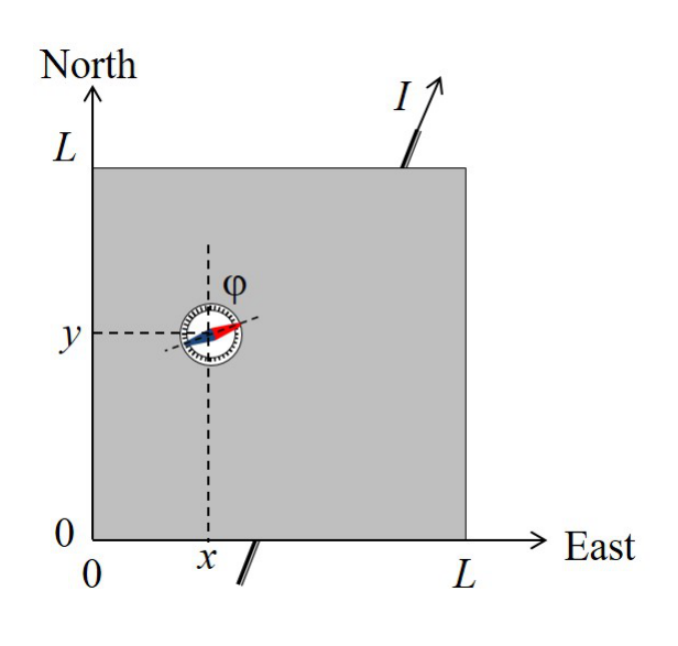
Grey square surface in the xy-plane with axes North (up) and East (right), corners marked 0 and L on both axes; the wire with current I enters under the bottom edge and leaves at the top edge; a compass at point (x, y) with dashed guide lines, its needle deflected by angle φ from the North direction.

The wire is connected to an adjustable DC source (not shown in the figure), which can provide a current $I$ in the range from $-5\ \mathrm{A}$ to $5\ \mathrm{A}$ . The reversal of the sign of the current corresponds to a reversal of the polarity of the source. A small compass can be placed on the square surface, (including its circumference) to sense the magnetic field of the wire through the deflection angle $\varphi$ between the magnetic needle and the North ( $y$ ) direction. Positive $\varphi$ values correspond to an Eastward deflection, as shown in the figure, while negative $\varphi$ correspond to a Westward deflection. You can assume that:

The magnetic needle is a point-like magnetic dipole, which can rotate freely around the vertical axis, i.e. the compass is sensitive to the horizontal component of the magnetic field only.
The height of the needle above the surface is negligible compared to the depth of the wire beneath the surface, i.e. the needle is situated in the $xy$ -plane.

Design your experiment and make the necessary simulations to perform the following tasks:

a. Determine the orientation of the wire with respect to the coordinate system by specifying its equation in the form: $y = ax + b$ , and estimate the uncertainties of the parameters $a$ and $b$ . Draw the wire position on a graph and indicate the direction corresponding to a positive current $I$ . [3 т.]

b. Determine the depth $h$ of the wire below the surface and the horizontal component $B_{\mathrm{E}}$ of the Earth's magnetic field. In this task you are not required to calculate the experimental uncertainties explicitly, however, your final results must be represented with an appropriate number of significant digits. [6 т.]

The magnetic permeability of free space is

\mu_0 = 4\pi \times 10^{-7}\ \mathrm{T\,m/A}.

Description of the simulation software

The command line program simulates the measurement of the deflection angle $\varphi$ after providing the current $I$ and placing the compass at the coordinates $x$ and $y$ on the surface.

A typical output of a single simulation cycle of the program looks like:

Enter I (A) between -5.0 and 5.0: 3.4
Enter X (mm) between 0 and 100: 55
Enter Y (mm) between 0 and 100: 31
PHI = -33 degrees
-------------------------------
Enter I (A) between -5.0 and 5.0: _

First, you enter the current $I$ in $A$ (the number between $-5.0$ and $5.0$ ), then coordinates $x$ and $y$ in $mm$ (the numbers between $0$ and $100$ ). Each input is confirmed with the Enter key. The program will output the value of $\varphi$ (PHI) in degrees (rounded to $1^{\circ}$ ) and return to the initial prompt.

The current input $I$ will be rounded to $0.1\ \mathrm{A}$ , the coordinate inputs $x$ , $y$ will be rounded to $1\ \mathrm{mm}$ before being used in simulation. (There is no point in trying to input more precise numbers).

Every time you change the position of a compass, its real position used in simulation differs from the input coordinates with an error about $0.5\ \mathrm{mm}$ . (It is a simulation of a limited precision when you place an object).

Any time you need to quit the program, press Ctrl+C.

Отговори

Решение

Theoretical background

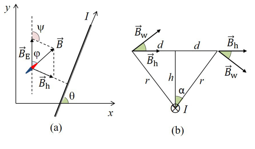
As shown in Fig. 1, the horizontal projection $\vec{B}_{\mathrm{h}}$ of the magnetic induction $\vec{B}_{\mathrm{w}}$ of the wire has the same direction and is perpendicular to the wire in all points of the $xy$ plane. It is clear that $\vec{B}_{\mathrm{h}}$ makes with North ( $y$ ) direction an angle $\psi = 180^{\circ} - \theta$ , where $\theta$ is the angle between the direction of the current and the positive $x$ -direction. The magnetic needle points along the vector $\vec{B} = \vec{B}_{\mathrm{h}} + \vec{B}_{\mathrm{E}}$ of the total magnetic induction. As evident from the vector triangle on Fig. 1(a), the deflection angle $\varphi$ can be obtained through the sine-theorem:

\frac{B_{\mathrm{h}}}{B_{\mathrm{E}}} = \frac{\sin\varphi}{\sin(\psi - \varphi)} = \frac{\sin\varphi}{\sin(\theta + \varphi)} \qquad (1)

Consider a point on the surface at a distance $d$ from the wire projection onto $xy$ plane, and at a distance $r = \sqrt{d^2 + h^2}$ from the wire, as shown in Fig. 1(b). It follows from the Ampère's law that the magnitude of magnetic induction of the wire at that point is

B_{\mathrm{w}} = \frac{\mu_0 I}{2\pi r} \qquad (2)

and the magnitude of its horizontal projection is

B_{\mathrm{h}} = B_{\mathrm{w}} \cos\alpha = \frac{\mu_0 I h}{2\pi(d^2 + h^2)}. \qquad (3)

Equations (1) and (3) are sufficient to complete all tasks of the problem.

(a) Vector triangle in the xy axes: the wire with current I at angle θ to the x-axis; at a point, B_E points North (y), B_h points perpendicular to the wire, their sum B makes angle φ with North; angle ψ between B_h and North. (b) Cross-section: wire (current I into the page) at depth h, two surface points at distance d on either side at distance r from the wire, angle α at the wire; vectors B_w and B_h drawn at each point. — Figure 1: Notations used in the derivation of the basic equations.

Graph of Y (mm) versus X (mm), both 0 to 100, with measured points with error bars and a red straight line falling from about y = 75 at x = 0 to about y = 17 at x = 100; an arrow on the line labelled I > 0 points towards increasing x. — Figure 2: $xy$ -projection of the wire with indicated positive $I$ direction.

Task (a): Determination of the horizontal position of the wire

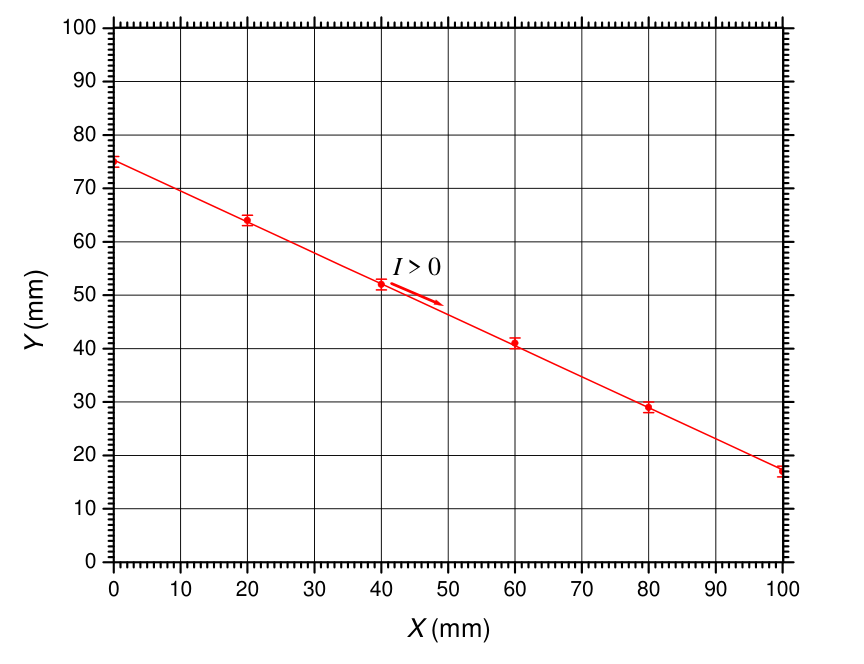
As evident from the vector triangle (Fig. 1), the maximum absolute value of the deflection angle at a given current is met at $d = 0$ where $B_{\mathrm{h}}$ is maximal, i.e. vertically above the wire. Therefore, the wire can be tracked by finding two or more points on the surface where $|\varphi|$ reaches a maximum. First, a coarse scan of the border with a step of, say, 10 mm, can be performed in order to locate intervals, where $|\varphi|$ goes through a maximum. In this way we establish that the wire projection crosses the West side ( $x = 0$ mm) at $y \in [60\ \mathrm{mm}, 90\ \mathrm{mm}]$ and the East side ( $x = 100$ mm) at $y \in [10\ \mathrm{mm}, 30\ \mathrm{mm}]$ . A finer scan of these intervals with a step of 1 mm allows to determine the approximate coordinates of the two crosspoints as $P_1 = (0.0{\pm}0.5, 75{\pm}1)$ mm and $P_2 = (100.0{\pm}0.5, 17{\pm}1)$ mm. The uncertainty of the $y$ coordinate is 1 mm since near the maximum $|\varphi|$ changes slowly and takes the same rounded value at three consecutive points. Additional scans along vertical (horizontal) lines of intermediate $x$ ( $y$ ) values could be done in order to find more points along the wire projection, and to determine the equation of the wire more precisely by means of a least-squares fit. A typical set of values is given in Table 1. The fitted equation of the wire is, respectively

y = ax + b = -0.58x + 75.3\ \mathrm{mm} \qquad (4)

with estimated parameter uncertainties of $\delta a \approx 0.01$ and $\delta b \approx 0.4$ mm. The parameter uncertainties scale as $1/\sqrt{N}$ , where $N$ is the number of experimental points. A graph of the wire projection in the $xy$ -plane is shown in Fig. 2. Since $\varphi < 0$ at $I > 0$ , the positive $I$ direction is from the West to the East border, as shown in the graph.

Table 1: Points, where $|\varphi|$ reaches a maximum of $143^{\circ}$ at a current $I = +5$ A.

$x$ (mm)	$y$ (mm)
0	75
20	64
40	52
60	41
80	29
100	17

Task (b): Determination of $h$ and $B_{\mathrm{E}}$

As follows from equations (1) and (3), the deflection angle $\varphi$ at a distance $d$ from the horizontal projection of the wire satisfies the equation

\frac{\sin\varphi}{\sin(\theta + \varphi)} = \frac{\mu_0 I h}{2\pi B_{\mathrm{E}}(d^2 + h^2)}. \qquad (5)

where the angle $\theta$ can be calculated from the slope coefficient $a$ of the wire:

\theta = \arctan(a) = -30.1^{\circ} \pm 0.4^{\circ} \qquad (6)

The distance $d$ between a point with coordinates $(x, y)$ and the wire projection can either be measured directly on the graph in Fig. 2, or calculated as:

d = |(ax + b - y)\cos\theta| \approx 0.865|ax + b - y| \qquad (7)

It follows from equations (5)–(7) that the unknown $h$ and $B_{\mathrm{E}}$ could be determined if the deflection angle $\varphi$ is measured in at least two points situated at different distances from the wire. However, due to the random error, associated with compass positioning and the rounding error of the angle reading, such a minimalist approach is quite inaccurate. Therefore, systematic measurements at several distances $d$ and/or different currents $I$ , are necessary to obtain sufficiently precise estimate for $h$ and $B_{\mathrm{E}}$ . Two generic approaches could be followed, as well as a combination between them.

Method I. Varying the current at fixed distances. By defining a new dimensionless variable $U = \sin\varphi/\sin(\varphi - 30.1^{\circ})$ , equation (5) is linearized as:

I = kU \qquad (8)

where the slope coefficient is:

k = \frac{2\pi B_{\mathrm{E}}(d^2 + h^2)}{\mu_0 h} \qquad (9)

Therefore, the unknown $B_{\mathrm{E}}$ and $h$ can be estimated after obtaining $k$ for at least two different distances $d$ from the wire. Table 2 summarizes the results of measurements at $d_1 = 0$ mm (vertically above the wire) and at $d_2 = 10$ mm in a point with coordinates $x = 20$ mm and $y = 75$ mm. Figure 3 shows the corresponding U-I graphs, and the estimated values of the slope coefficients are also listed in the table 2.

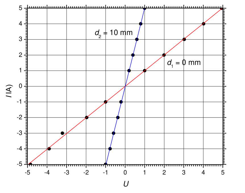
Graph of I (A) from -5 to 5 versus U from -5 to 5 with two straight fit lines through the origin: a red line of slope about 1 labelled d1 = 0 mm and a steep blue line of slope about 5 labelled d2 = 10 mm, with the data points on each. — Figure 3: U-I graphs for two different distances $d$ from the wire, and the corresponding linear fits.

Table 2: Experimental data for the deflection angle $\varphi$ vs. current $I$ at two different distances $d$ .

(0 mm,75 mm); $d_1 = 0$ mm			(20 mm,75 mm); $d_2 = 10$ mm
$I$ (A)	$\varphi$ (deg)	$U$	$I$ (A)	$\varphi$ (deg)	$U$
-5.0	25	-4.85	-5.0	15	-1.00
-4.0	24	-3.89	-4.0	13	-0.77
-3.0	23	-3.21	-3.0	11	-0.59
-2.0	20	-1.97	-2.0	8	-0.37
-1.0	15	-1.00	-1.0	5	-0.21
1.0	-75	1.00	1.0	-7	0.20
2.0	-126	1.99	2.0	-17	0.40
3.0	-137	3.03	3.0	-32	0.60
4.0	-141	4.02	4.0	-52	0.80
5.0	-143	4.94	5.0	-75	1.00
$k_1 = 1.01 \pm 0.01$ A			$k_2 = 5.04 \pm 0.03$ A

It follows from equation (8) that:

\frac{B_{\mathrm{E}}}{h} = \frac{\mu_0(k_2 - k_1)}{2\pi(d_2^2 - d_1^2)} = 8.06 \times 10^{-6}\ \mathrm{T/mm} \qquad (10)

and

B_{\mathrm{E}} h = \frac{\mu_0(d_2^2 k_1 - d_1^2 k_2)}{2\pi(d_2^2 - d_1^2)} = 1.98 \times 10^{-4}\ \mathrm{T \cdot mm} \qquad (11)

Alternatively, one can also use

h = \sqrt{\frac{d_2^2 k_1 - d_1^2 k_2}{k_2 - k_1}} = 5.0\ \mathrm{mm}. \qquad (12)

Finally, we obtain for the horizontal component of the Earth's magnetic induction:

B_{\mathrm{E}} = 4.0 \times 10^{-5}\ \mathrm{T} \qquad (13)

and for the depth of the wire:

h = 5.0\ \mathrm{mm} \qquad (14)

These estimates of $h$ and $B_{\mathrm{E}}$ coincide with accuracy of two significant digits with the values preset in the simulation program.

Method II. Fixed current, varying the distance. Equation (5) can be rewritten in the form:

\frac{\sin(\theta + \varphi)}{\sin\varphi} = \frac{2\pi B_{\mathrm{E}}}{\mu_0 I h} d^2 + \frac{2\pi B_{\mathrm{E}} h}{\mu_0 I} \qquad (15)

which can be linearized by setting new auxiliary variables: $U = d^2$ and $V = \sin(\varphi - 30.1^{\circ})/\sin\varphi$ . A typical data set for this method is given in table 3, while the linearized U-V plot is shown in Fig. 4.

Table 3: Experimental data for the deflection angle $\varphi$ vs. distance $d$ at a fixed current $I = 5.0$ A.

$x$ (mm)	$y$ (mm)	$d$ (mm)	$\varphi$ (deg)	$U$ (mm $^2$ )	$V$
0	75	0	-143	0	0.203
2	75	1	-142	1	0.226
4	75	2	-142	4	0.226
6	75	3	-139	9	0.291
8	75	4	-138	16	0.311
10	75	5	-132	25	0.416
12	75	6	-128	36	0.475
14	75	7	-123	49	0.541
16	75	8	-111	64	0.674
18	75	9	-98	81	0.796
20	75	10	-79	100	0.963

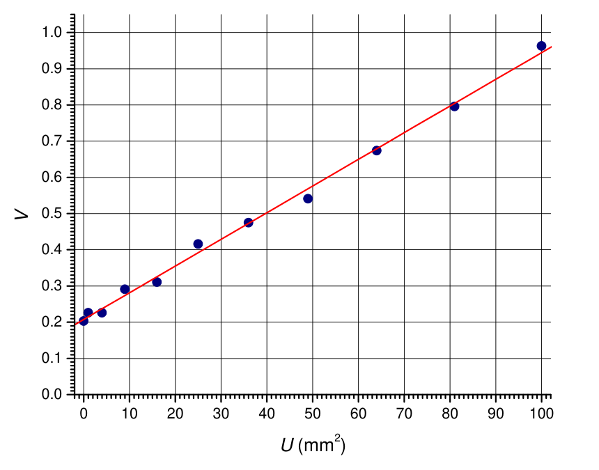
Graph of V from 0.0 to 1.0 versus U (mm²) from 0 to 100 with eleven data points and a red rising straight fit line from about 0.21 at U = 0 to about 0.95 at U = 100. — Figure 4: U-V graph obtained at a fixed current $I = 5.0$ A.

From the fitting line we obtain:

V = 7.37 \times 10^{-3}\mathrm{mm}^{-2} U + 0.208 \qquad (16)

which means $2\pi B_{\mathrm{E}} h/(\mu_0 I) = 0.208$ and $2\pi B_{\mathrm{E}}/(\mu_0 I h) = 7.37 \times 10^{-3}\mathrm{mm}^{-2}$ . Thus, we obtain:

B_{\mathrm{E}} = 3.9 \times 10^{-5}\ \mathrm{T} \qquad (17)

for the horizontal component of Earth's magnetic induction, and

h = 5.3\ \mathrm{mm} \qquad (18)

for the depth of the wire. These estimates are close to, but less accurate than the values obtained by Method I. The reason is that at small $d$ , there is a large relative error associated with wire positioning, i.e. with variable $U$ . At large $d$ , however, the deflection angle is small, and there is significant relative error, associated with the compass reading, i.e. with $V$ parameter.

Marking scheme

The basic equations could be stated in a separate section of the solution, or spread over different parts of the solution.

	Theoretical background	Points
T1	States explicitly or shows on a clear graph that the magnetic needle points along the total magnetic induction.	0.1
T2	Derives eq. (1) or equivalent.	0.3
T3	Writes down the Ampere's law (2).	0.2
T4	Derives eq. (3) or equivalent.	0.4
Total on Theory		1.0

In tasks A and B points for obtaining final results are given on an additive basis. If a given quantity, say $a$ -parameter of the line, falls into the widest interval, a minimum number of points is given. If the value, however, belongs to the subsequent narrower interval, annotated points are added to the points for the previous interval, and so on, down to the narrowest interval.

	Task A: Horizontal position of the wire	Points
A1	State or use that the wire is located where $\lvert\varphi\rvert$ is maximal.	0.2
	(state alternative method which allows to find only $a$ );	(0.1)
A2	Find points on the wire at most 2mm away from both cross points with the border.	0.2
A3	Find $n$ points along the wire projection:
	$n = 3$ or 4;	0.3
	$n \geq 5$ .	0.5
A4	Draw wire projection on the graph:
	plot all measured points or at least 5;	0.2
	if a point drawn incorrectly;	-0.1
	line through the points;	0.2
	axes labels and units;	0.1
	axes tick marks with values;	0.1
	correctly indicated positive $I$ direction.	0.3
A5	Equation of the line:
	$a$ within [-0.61;-0.55];	0.1
	$a$ within [-0.60;-0.56];	+0.1
	$a$ within [-0.59;-0.57];	+0.3
	$b$ within [73.6;77.0] mm;	0.1
	$b$ within [74.6;76.0] mm;	+0.1
	$b$ within [74.9;75.7] mm .	+0.3
	Correctly estimated uncertainties of $a$ and $b$ .	0.2
Total on Task A		3.0

Since there are several approaches to the solution of Task B, the subsequent marking scheme is unified in order to fit all methods of solution. The data point is defined as a single measurement of $\varphi$ at given $I$ , $x$ , and $y$ . The data point weight $W$ is defined as a mark related to the way, in which the measured data are presented and treated numerically:

$I$ , $x$ , $y$ , and the corresponding $\varphi$ are documented in a table with appropriate number of digits.	0.1
The value of the distance $d$ to the wire, and the values of the auxiliary linearizing variables (if required by the solution) are calculated correctly and documented in the table.	0.1
Maximum $W$	0.2

The total mark for data recording and treatment (B2, see the table below) scales linearly with the number of data points $N$ for up to $N = 8$ . All data points after 8-th do not contribute to the total mark on B2. Data points measured in part A only count towards the mark of B2 if it is stated in part B that they can be used for this part as well, or if they are used implicitly.

	Task B: Finding $B_{\mathrm{E}}$ and $h$	Points
B1	Makes appropriate choice of auxiliary variables, which linearize eq. (3) OR derives explicit expressions for $B_{\mathrm{E}}$ and $h$ in terms of two measured angles $\varphi$ at two different distances $d$ (minimalist approach).	0.6
B2	Data recording and treatment:
	$\min(N, 8) \times W$	1.6
B3	Organization of data in table(s):
	Column titles	0.2
	Units	0.2
B4	Extracting parameters
	Graphical method:
	For plotting $n$ points $m = \min(n, 8)$	0.1 $m$
	Coverage of at least 75% of the graph window	0.2
	Titles on axes	0.2
	Units on axes	0.2
	Tick marks with annotated values	0.2
	Fitting line(s) is (are) drawn on the graph(s)	0.5
	Fitting line parameters are extracted and explicitly stated	0.5
	Linear regression without graph:
	using $n$ points $m = \min(n, 8)$	0.1 $m$
	correct fit	1.8
	Averaging over $n$ two-point measurements: $m = \min(n, 13)$	0.2 $m$
B5	Final values of $B_{\mathrm{E}}$ and $h$ are calculated from the line parameters or calculated from the results of a two-point measurement (minimalist approach):
	$B_{\mathrm{E}} \in [3.7; 4.3] \times 10^{-5}$ T	0.1
	$B_{\mathrm{E}} \in [3.8; 4.2] \times 10^{-5}$ T	+0.1
	$B_{\mathrm{E}} \in [3.9; 4.1] \times 10^{-5}$ T	+0.2
	$h \in [4.5; 5.5]$ mm	0.1
	$h \in [4.7; 5.3]$ mm	+0.1
	$h \in [4.9; 5.1]$ mm	+0.2
Total on Task B		6.0

Оригинал в Архива: EuPhO_2021-exp.pdf · официални решения: EuPhO_2021_exp_solutions-2.pdf