EuPhO 2025, Теория — Задача 2. Floating table
Theoretical Problems. Language: English · 10 т.
Условие
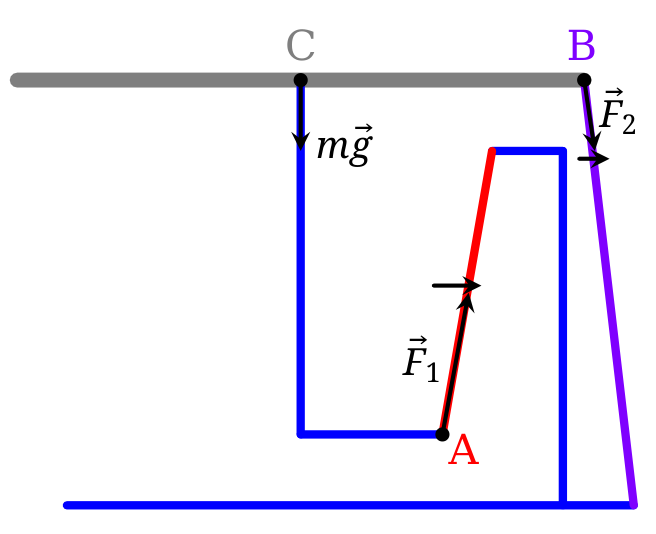
A table is made by fastening a metal frame to a massive uniform plate (so they form a rigid body) and attaching it with chains to another frame that is fixed on the horizontal ground. The motion of the table is limited to the plane of the side view (right picture).
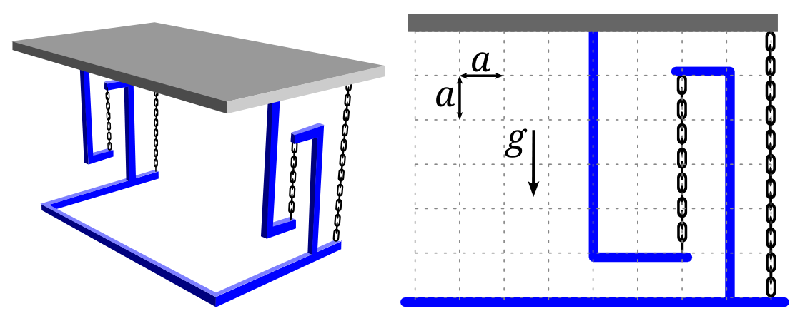
a) Show that in the configuration on the side view, the table is in a stable equilibrium. [4 т.]
b) Find the period of the small oscillations. [6 т.]
The masses of the chains and the frame can be neglected. The chains are frictionless, inextensible, and remain tensioned in oscillations. The grid step is , the acceleration of gravity .
Решение
Solution with forces First, let us consider the forces and torques and show that in the configuration shown in the figure, the table is indeed in equilibrium. By the word “table”, we understand the rigid body formed by the plate and the frame attached to it. In the following considerations and descriptions of the table position we often use positions of points A, B and C, which belong to the rigid table: distances between them do not change. Since in the problem statement, the motion is limited to the side view only, the pair of short chains will always have the same position when viewed from the side. So we will consider them as a single chain (chain 1) with the tension doubled. The same is true for the pair of long chains (chain 2).
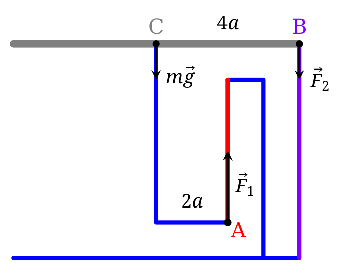
There are 3 forces acting on a table (see Fig. 3): plate weight (at the center of mass of the table C), and 2 tension forces from the chains: (at point A, chain 1) and (at point B, chain 2). Since all the forces only have vertical components different from 0, their horizontal components are balanced and for their vertical components, the balance equation is:
Finally, consider the torque balance around the point :
Solving the system of equations (8-9), we get and . Since both , we conclude that the chains are indeed tensioned and the system is in equilibrium.
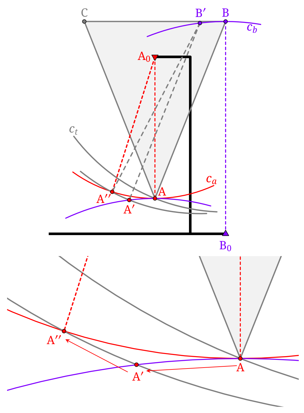
Now let's analyze how the table rotates, when it is displaced. Since the chains are tensioned and inextensible, the point can only travel along the circle . Similarly, the distance between the point and any point inside the circle is smaller than the length of the short chain (4a); the distance between the point and any point outside of the circle is larger than .
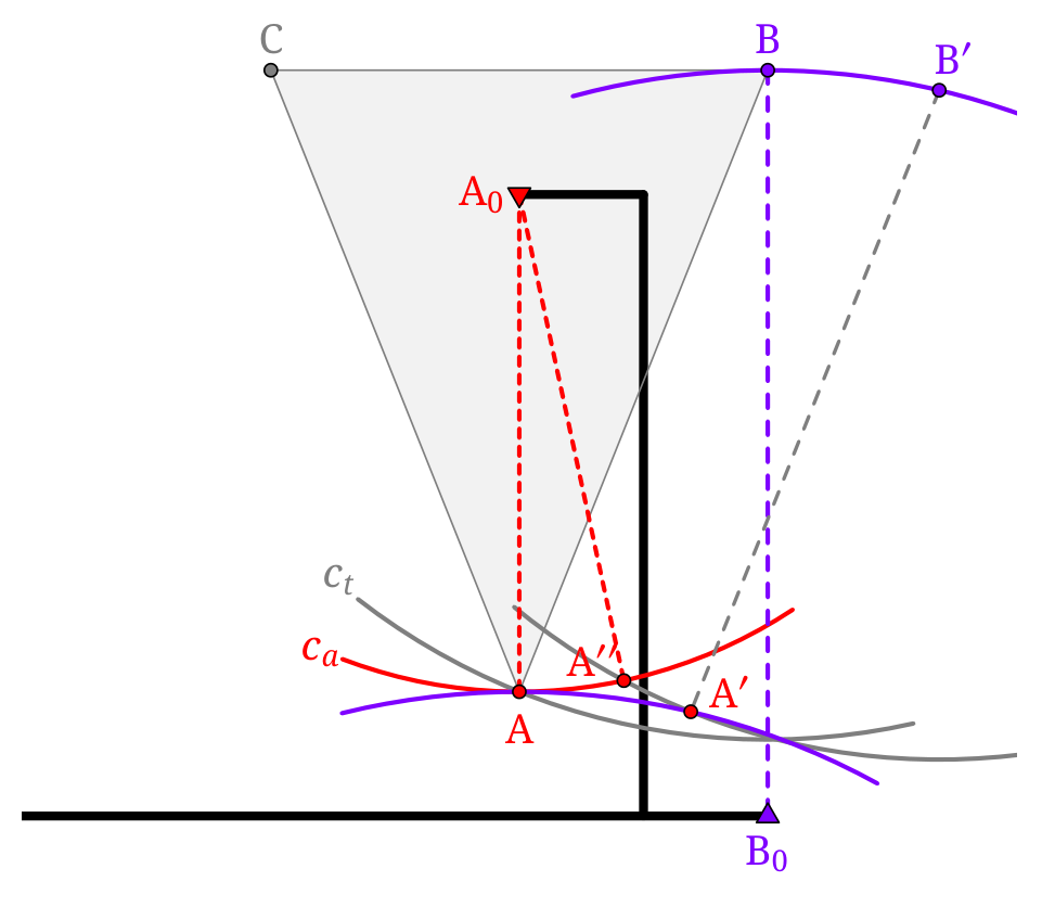
Since the table is rigid, if we fix the point B and rotate the table around it, point A would travel along the circle . From the way how intersects with , we can conclude that if the table is rotated clockwise, the distance decreases. And if it is rotated counter-clockwise, increases.
Let's imagine we translate (move without rotation) the table to the left, so the point travels to the point . Point would move to the point , as shown in Fig. 4. Since is outside of the circle , and the table has to rotate clockwise (around B') to compensate for this change and return the point back to the circle (point A'') to satisfy the constant chain length constraint.
If we translate the table in the opposite direction, following similar arguments, we find that the table rotates clockwise in this case too, see Fig. 5.
Since the table rotates in the same direction for both positive and negative horizontal displacements, the Taylor expansion of the angle of rotation does not contain a linear term in : . This means that for small horizontal displacements, we can neglect the table rotation.
Let's look at what happens when the table is displaced infinitesimally from its initial position in the horizontal direction (it will also move in the vertical direction, but the displacement in the vertical direction is an order of magnitude smaller and we will neglect it). The vertical components of the forces in the chains do not change significantly, but as you can see in the Fig. 6, the horizontal components of the forces in both chains appear in the direction opposite to the displacement. This means that the equilibrium is stable.
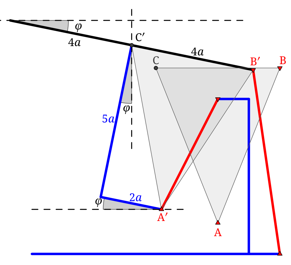
Since we have already drawn a figure showing the displaced position of the table, let us write the equation of motion for the table plate for small horizontal displacements , where and are small angles between the chains 1 and 2 respectively and the vertical. Since the table displacement is small, tension forces and cannot change significantly (the force change is of the same order as the displacement). Thus, we can use the previously found values:
where we have also considered the lengths of the chains (chain 1) and (chain 2), neglected the rotation of the plate and used small angle approximations. Rearranging this equation, we get:
which describes horizontal oscillations of the table plate with , frequency and period
Solution with energies Let's denote the small displacement of the centre of mass from equilibrium position C to C′ as , where , and the small tilt of the table as , as shown in Fig. 7.
Given the small angle approximation ( and ), the displacement of points from equilibrium positions A and B to A′ and B′ are:
Now we can write a condition that the squared length of the small chain remains the same:
Let's notice that the largest term in is and in and , it's . Thus, we can omit all other terms, since they are of the higher order (and therefore smaller):
Doing the same for the long chain we get:
Omitting higher order terms we get:
Solving (10) and (11) as linear equations on and , we get:
Since the potential energy of the table
doesn't have a term linear in , we conclude that the system is in equilibrium. And since the coefficient for is positive, the equilibrium is stable.
The kinetic energy of the table is:
where is a moment of inertia with respect to rotation around the axis through the centre of mass C. Since both and depend on , their squared derivatives will be proportional to and can be neglected when compared to term.
Finally, we can find the period of oscillations from the ratio of coefficients of (13) and (12):
Solution with the curvature We begin with the observation that at the initial horizontal position, points A and B in Fig. 3 move horizontally. Therefore, the instantaneous centre of table's rotation is at infinity (found as the intersection of lines perpendicular to the velocity vectors, which are parallel in this case), or in other words there is no rotation. Another way to see it is to consider the projections of the velocities and to the line which should be the same in a rigid body. Thus and all the points of the table move with the same velocity, i.e. there is no immediate rotation.
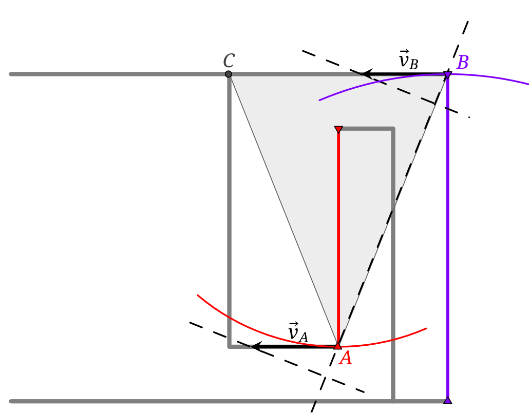
Consequently, no rotational kinetic energy is involved, and the motion of the table can be treated as the motion of a point mass located at the centre of mass, point C. Since at the given configuration, the can only be horizontal, we conclude that initially table is at equilibrium. All that remains is to find the radius of curvature of its trajectory and calculate .
To find the radius of curvature, we note that for an arbitrary point on the table, the curvature of its trajectory is a linear function of its coordinates, where denotes a unit vector pointing towards the centre of curvature. Indeed, using a non-inertial reference frame where the rigid body remains at rest with origin at O, the acceleration of a point is the superposition of: the acceleration of , the centripetal acceleration , and the tangential acceleration . All of these are linear functions of the coordinates of point , where denotes the angular acceleration and the angular speed. Hence, in the lab frame, the acceleration of point is a linear function of coordinates, as must be its centripetal acceleration . Since the angular speed of the table is zero, all points move with the same speed, so must be a linear function of coordinates.
The remaining calculation is straightforward: due to the translational motion of the body, curvatures depend only on the horizontal coordinate . The curvature of at is , with the minus sign indicating that the vector points downwards. The curvature of at is . Hence, the curvature of is , giving and resulting in . Positive curvature means that the position is a stable equilibrium.
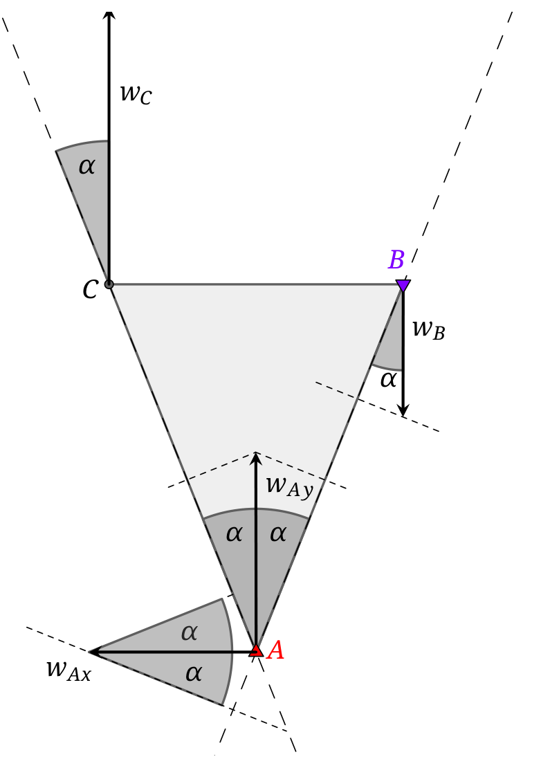
Another way to see it, is to consider normal acceleration of point C. For 2 points of a rigid body and , the projections of their accelerations , to the segment differ by the value . However, in our case since there is no rotation, the projections of acceleration are equal (like velocities). This means that the acceleration is also normal and equal to . Point A has both normal and tangential acceleration. Comparing projections of points , , and , , we get:
Thus, we find that
so radius of curvature is .
You can visualize the motion of the table using a GeoGebra tool, following the web link or the qr code https://www.geogebra.org/m/wbqwp3tf
Marking scheme T2
| Pts | ||
|---|---|---|
| A | Table is in equilibrium. Partial points: (1pt) Sketch of forces or eqn for forces | 2.0 |
| B | The equilibrium is stable. Partial points: (1pt) Sketch with returning forces, but there is no proof that ; (1pt) There is a statement that the stability comes from if , but is not found correctly (and thus could potentially be negative) | 2.0 |
| C | Table can rotate: whether it is clear from the sketch or from the equations, i.e. is introduced | 1.0 |
| D | Table does not have immediate rotation whether it is proved separately or follows naturally from the results of calculations: geometry considered ; eqn for constraints ; immediate velocities no rotation | 1.0 |
| E | The plan how to find the period of oscillation: 2nd Newton's law ; idea to find kinetic and potential energies; using the curvature of the trajectory | 1.0 |
| F | Finding all the elements for the plan above: small horizontal forces; energies to the correct approximations; accelerations/curvatures. Partial points: (1pt) if not all elements are found or they are found with mistakes; (1pt) if there is no proof (or no consideration about the rotation at all), but other than that, everything is correct; (0pts) if some elements are there, but the plan was different (e.g. the student was looking for energies, but has the expression for forces) | 2.0 |
| G | Formula and number for . Partial points: (0.5pts) only formula or a number; (0.5pts) simple mistake (like inverse formula under the root) | 1.0 |
| Total | 10.0 |

- Only a single partial point is applied (whatever is larger)
- If there is a single simple arithemetic error/typo in calculations in item F, which leads to a wrong formula value in item G, then F and G receive 1 pt each (no propagation of error). This doesn't apply to more profound errors in physics/geometry
Оригинал в Архива: eupho2025_theory_problems.pdf · официални решения: eupho2025_theory_solutions.pdf