EuPhO 2025, Теория — Задача 3. Crossed wires
Theoretical Problems. Language: English · 10 т.
Условие
a) Current flows through an infinite, straight, thin wire. There is an externally imposed, uniform magnetic field directed parallel to the wire. Qualitatively sketch one of the magnetic field lines. [1 т.]
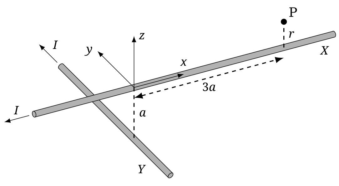
b) Now consider two infinite, straight, thin wires (wires and ), each carrying a current as shown in the figure. The -axis coincides with wire , while wire is parallel to the -axis and passes through the point . Let P be the point . Assuming , calculate , the distance of closest approach of the magnetic field line that passes through P to the wire . [5 т.]
c) Let be the length of this field line between P and its point of closest approach to wire . Using values and , calculate to within 20% relative error. [4 т.]
Отговори
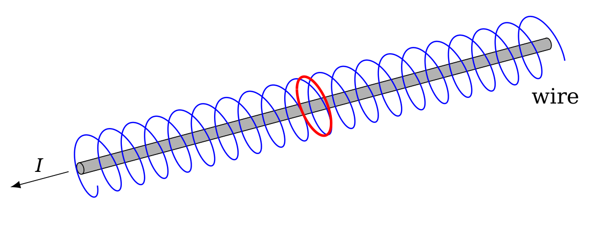
a) Field lines become a helix around the wire when an external field with a component parallel to the wire is added.
b)
c) 179 m
L ≈ 17.9 a²/r ≈ 179 m; marking scheme accepts 140 m ≤ L ≤ 215 m.
Решение
Part a) In the absence of an externally imposed magnetic field, an infinite, straight, thin wire creates a magnetic field whose field lines are closed circular loops. These loops lie in the plane perpendicular to the wire and are centered on the wire (red circle in the figure).
Now, consider the effect of introducing the externally imposed magnetic field. At any point, the total magnetic field is the vector sum of the magnetic field of the wire and the externally imposed magnetic field. The total magnetic field now has a component parallel to the wire. This means the magnetic field lines do not remain in a plane perpendicular to the wire. They do not form closed loops any more. Instead, they will spiral around the wire, tracing out a helix (blue curve in the figure).
Part b) It is a standard result that the magnetic field around an infinite, straight, thin wire carrying a current has magnitude , where is the perpendicular distance to the wire. This magnetic field strength increases as decreases. Before considering the wire configuration of part b, it will be useful to discuss what happens in part a if the helical field line is very close to the wire. By 'close', we mean values of small enough that the magnetic field of the wire is much greater than the externally applied magnetic field. Then, the field lines cannot deviate much from the circular loops they would trace out if the externally applied field were not present. This means the helix would be wound very tightly.
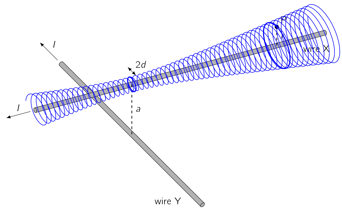
Now we move on to discuss the wire configuration of part b. Let the magnetic field due to wire be and the magnetic field due to wire be . At any point in space, the magnetic field is the vector sum of and . At points that are close to wire (distances ), we have . Therefore, as in part a, the field lines near wire will not deviate very much from circular loops centered on wire . However, has a component along wire , so the field lines do not perfectly close on themselves. Instead, they will trace out a tightly wound spiral around wire , as shown in the figure for the previous part. Unlike there, the spiral is not necessarily a perfect helix: as the field lines spiral to larger or smaller , the radius of the spiral might change. To find the distance of closest approach of a field line to wire , we must find the minimal value of as varies.
The spiraling field line shown in the figure below seems to trace out a surface, , surrounding wire . A more precise definition of is as follows. Let be the circle of radius , centered on wire , in the plane . Through every point on , we can draw a magnetic field line. The set of field lines passing through points of traces out a surface; this is the surface we define as . Each field line in this set spirals around wire as described above, so looks like a 'funnel' whose cross section, at any fixed , is nearly circular. The cross section is nearly circular as long as the condition is satisfied, because this means the magnetic field is perturbed only slightly by wire and the field lines do not deviate much from the circular loops that they would trace if wire were not present. Near point P, is satisfied because . We will verify a posteriori that the magnetic field line never reaches values of that violate the condition .
The key idea is that the magnetic flux through the middle of the 'funnel' is conserved. No magnetic flux exits through the sides of the funnel because—by construction—the magnetic field is tangent to at every point. For this reason, the region bounded by is called a 'flux tube'. The flux through the flux tube is entirely due to , which is approximately uniform over the circular cross section at each .
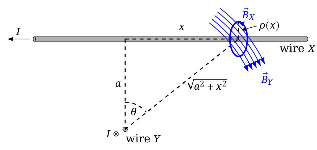
The component of directed along the wire is (see figure above). Therefore, the conserved flux is . The equation of is then , using the fact that passes through P. We can now see that never grows so large that fails, so our equation for remains valid for all . Then, the minimal value of is .
Part c) Let the point of closest approach be Q. We need to calculate the length of the spiraling field line between points P and Q. Due to the tight winding of the field lines, this length is much larger than or . Therefore, the precise position of point Q around the loop closest to (for example, whether it is on the side closer to wire or on the side further from wire ) is unimportant. To leading order, equals the length along the field line from P to the point on the field line with .
Consider two points on the field line whose -coordinates differ by a small amount . The length of the short segment of field line joining these points is given by . Here, we have decomposed the magnetic field vector into a component along wire and a component perpendicular to wire . In the previous part, we found . The field of wire gives the dominant contribution to , so . These expressions are approximate and ignore corrections of order . Since , ignoring these corrections is acceptable for the required accuracy of 20%. The total length is obtained by integration:
Now, we use the equation for derived in part b: . The result is
This expression must be numerically evaluated to within 20% relative error. To obtain a numerical value for the integral, we could use the trapezium rule or we could draw the curve between and on graph paper and count the number of squares beneath the curve. In fact, a crude estimate using a single trapezium is sufficient for the required accuracy: , resulting in a length of m. The exact result is m.
Although not necessary for full credit, it is possible to evaluate the integral exactly. Substituting with and using gives
Now, we use to obtain
Finally, we use and to find
This gives m, as stated above.
Marking scheme T3
Problem T3 a)
| Pts. | ||
|---|---|---|
| A | draw clear sketch (straight wire, smooth field line, ...) | 0.2 |
| field line … | ||
| B | …is not closed | 0.2 |
| C | ...is periodic in | 0.2 |
| D | ...is helical (only 0.1 if chirality is wrong) | 0.2 |
| E | ...is centered on wire | 0.2 |
| Total on T3 a) | 1.0 |
Problem T3 b)
| Pts. | ||
|---|---|---|
| A | state or derive formula for magnetic field of infinite, straight wire (only 0.2 if direction is not clear) | 0.4 |
| sketch or explain shape of field line | ||
| B | field line is locally nearly circular | 0.2 |
| C | field line resembles helix tightly wound around wire | 0.2 |
| D | radius of helix is changing | 0.3 |
| E | idea to consider funnel surface | 0.5 |
| F | realize and justify that -flux is conserved along funnel | 1.0 |
| G | argue or show that radius of flux tube is smallest at | 0.5 |
| H | approximate as uniform in flux tube cross-sections | 0.4 |
| I | determine flux at (0.3 for projection, 0.2 for area) | 0.5 |
| J | determine flux at using | 0.3 |
| K | calculate final result for | 0.5 |
| L | check of validity of approximations in considered region | 0.2 |
| Total on T3 b) | 5.0 |
Problem T3 c)
| Pts. | ||
|---|---|---|
| A | realize that is much larger than and (also if implicit) | 0.2 |
| B | equate with using -field components or an angle | 0.4 |
| C | realize that is dominated by wire (might be mentioned in part b) already) | 0.3 |
| D | derive integral expression for | 0.4 |
| E | provide expression for in terms of , and (also if in part b)) | 0.5 |
| F | carry out reasonable numerical approximation or rigorous calculation of integral | 1.2 |
| G | result with 140 m 215 m (-0.2 if # significant figures is 1 or > 3) | 1.0 |
| Total on T3 c) | 4.0 |
General rules for marking in T3:
- The grain size for marking is 0.1 Pts.
- Partial marks can be awarded for most aspects.
- For each mistake in calculation (algebraic or numeric) 0.2 Pts. are deducted.
- If a mistake leads to a dimensionally incorrect expression no marks are given for the result.
- Propagating errors are not punished again unless they are dimensionally wrong or entail oversimplified/wrong physics (e.g. neglecting friction effects).
- In cases, where in part b) the distance of closest approach is determined by using an approximation that only considers the -field close to P (or any similar simplification), the following maximum marks can be obtained: A to C - 0.2 each, E - 0.3 for the idea to determine from a local consideration, H - 0.4, K - 0.3 for a simplified calculation of . Total: max. 1.6 Pts.
Оригинал в Архива: eupho2025_theory_problems.pdf · официални решения: eupho2025_theory_solutions.pdf