Съдържание

IAO 2016, Практически тур, Група β — Задача 6. The first gravitational wave detection

Оригинал на условието (PDF)Съобщи за грешка

Всички материали от IAO 2016

XXI International Astronomy Olympiad. Practical round. Group β · 5 октомври 2016 г. · 12 т.

Условие

In 1916, the year after the final formulation of the equations of general relativity, Albert Einstein predicted the existence of gravitational waves. They are emitted by accelerating masses in a way similar to the emission of electromagnetic waves by accelerating charges. In the case of gravity, like electromagnetism,.when a stationary mass moves suddenly then the gravitational force exerted by it on the test masses changes. However, that change will not happen immediately. Instead, the information that the mass moved will propagate at the speed of light and will take the form of gravitational radiation. When the gravitational wave reaches the test masses, those test masses accelerate, because the gravitational force suddenly changes. For a mass undergoing periodic motion, the gravitational waves it produces will be periodic, and those can accelerate surrounding test masses periodically.

On September 14, 2015, the two detectors of the Laser Interferometer Gravitational-Wave Observatory (LIGO) detected the coincident signal GW150914 as shown in Fig. 1. It was the first direct detection of gravitational waves and the first direct observation of a binary black hole system merging to form a single black hole. The distance to the merging black hole binary system was determined to lie somewhere between 250 and 600 Mpc, and the two initial black hole masses as being $36\pm4\ M_{\odot}$ and $28\pm4\ M_{\odot}$ , respectively. When those two black holes merged, they formed a single black hole of mass $62\pm4 M_{\odot}$ . The missing mass was emitted as energy in gravitational radiation, which was calculated to be $3.0\pm0.5\ M_{\odot}c^2$ . As usual, $1\ M_{\odot}$ is one solar mass equal to $2.0\times10^{30}\mathrm{kg}$ , and $c = 3.0\times10^{8}\ \mathrm{m/s}$ is the speed of light in vacuum. The peak emitted power of gravitational radiation was calculated at several times of $10^{49}\ \mathrm{W}$ – more than 10 times greater than the combined power of all light radiated by all the stars in the observable universe.

Graph printed rotated by 90 degrees: strain h/10^-21 (from -1.0 to 1.0) against time t(s) from about 0.25 to 0.46 s, with ticks at 0.30, 0.35, 0.40 and 0.45. Two oscillating curves, blue for Livingston, Louisiana and orange for Hanford, Washington (legend), grow in amplitude and frequency up to about 0.42 s and then die out. Pictures of two orbiting black holes marked (1), a merging pair marked (2) and a single black hole marked (3) are placed along the time axis. — Fig. 1. The gravitational-wave event GW150914 observed by the two LIGO detectors. The vertical axis shows the amplitude of the gravitational wave (the strain, h). The black holes go through the following stages (images placed along the horizontal axis at their roughly corresponding times): (1) the inspiral, as the two black holes approach each other; (2) the merger, as the black holes join together; and (3) the ringdown, as the single black hole that has newly formed briefly oscillates before settling down.

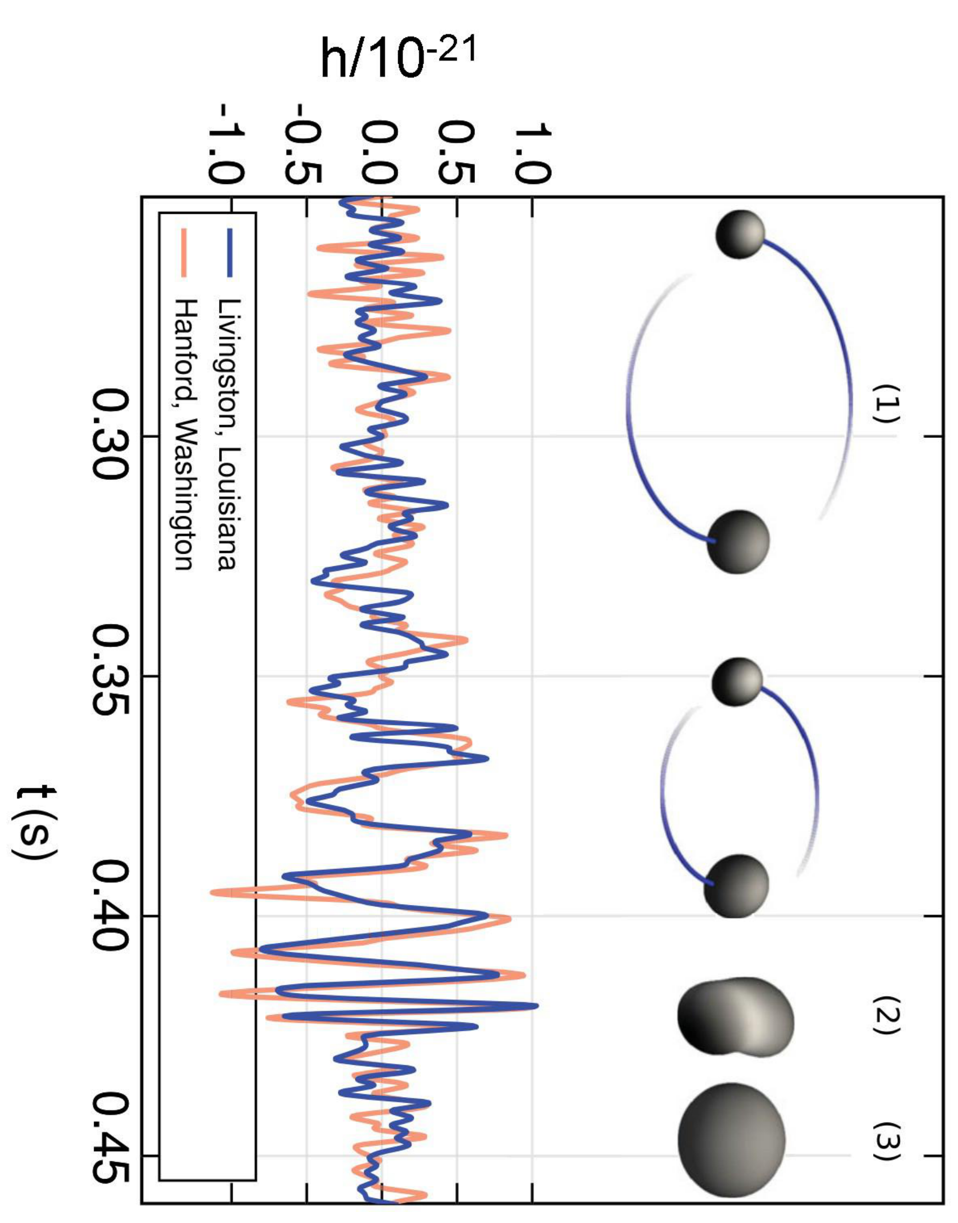
Due to the tidal forces gravitational waves cause relative displacements ( $\Delta L$ ) in the test masses that are proportional to the distance ( $L$ ) between those test masses. Physicists define the amplitude of gravitational waves by using the dimensionless quantity $h$ , defined as

h = \Delta L/L

which is usually called the dimensionless strain of the gravitational wave. This is the quantity plotted on the vertical axis of Fig.1.

Using a Newtonian (classical) mechanics approximation do the following tasks:

6.1. Using the masses quoted by the LIGO team, calculate the radii of the horizons of the two black holes before they merged. Include an estimate of the error for the radii.. [1 т.]

6.2. From the measurements of the gravitational wave signal presented in the graph above, find the orbital period of the black hole binary at the moment of the merger. [2,5 т.]

6.3. Estimate the total mass of the initial black hole binary. Use only information of the observed gravitational radiation from the graph. Do not use any of the other LIGO results quoted above. [2 т.]

6.4. Find an expression for the energy released in gravitational waves until the time of the black hole merger in terms of the initial black hole masses ( $M_1$ and $M_2$ ) only. Using the result from 6.3., calculate the total released gravitational energy if you assume $M_1 = M_2$ . [1,5 т.]

6.5. Find the average power $P$ of gravitational wave emission during the last $0.10\mathrm{s}$ before the merger. [2 т.]

6.6. As with most waves, the gravitational wave flux is proportional to the square of the amplitude of the wave. The amplitude (strain) right next to the two merging black holes is approximately $h = (v/c)^2$ , where $\boldsymbol{v}$ is the orbital velocity of the black holes. Estimate the distance to the merging black holes detected by LIGO. [2 т.]

6.7. The LISA experiment aims to measure gravitational waves from colliding supermassive black holes at high cosmological redshift. Estimate the required sensitivity of LISA in terms of the dimensionless strain. [1 т.]

Отговори

Решение

The gravitational constant is γ or $G = 6.67\mathrm{x}10^{-11}\ \mathrm{m^3\ kg^{-1}\ s^{-2}}$

Problem β-6. The first gravitational wave detection.

6.1. 1 pt

The initial masses of the two black holes are $36+/-4M_{\odot}$ and $28+/-4M_{\odot}$ . Their Schwarzschild radii are calculated using $R_s = 2GM/c^2$ , which gives 107+/-12 km and 83+/-12 km. The errors are calculated using ( $\Delta R_s/R_s = \Delta M/M$ ).

6.2. 2.5 pts

A good estimate of the precision of the measurements can be gained by comparing the Hanford and Livingston signals. At the time of the merger, we see two strong maxima and a minimum of the signal. For them, the time-axis intercepts for the Livingston signal are approximately at:

[0.4190, 0.4215, 0.4234, 0.4259] s

while for the Hanford signal, they are at:

[0.4193, 0.4217, 0.4239, 0.4259] s

These correspond to half-periods of:

[0.0025, 0.0019, 0.0025] sec
[0.0024, 0.0022, 0.0020] sec

for the two signals, respectively.

Assuming those measurements are both independent and representative for the time of the merger, taking the average and standard deviation of those, we get the half-period of the signal to be:

$0.0023\pm0.0003\mathrm{s}$

An attempt at a more accurate determination can be made by building a P(t) diagram.

The signal has close to symmetric minima and maxima, and the trends of both the maxima and the minima are consistent across both the odd and even peaks. This symmetry implies that the signal is emitted from a binary system with two components of roughly equal masses, as confirmed by the LIGO results.

Therefore, from the symmetry of the configuration of the system, the signal must be identical irrespective of which of the initial black holes is closer to us while they orbit each other. Thus, the signal must have a period of exactly half of the orbital period of the black holes. Therefore, the orbital period at the time of the merger must be 4 times larger than the half-period of the signal quoted above.

Thus, we can conclude that the orbital period is:

$T = 0.0092 \pm 0.0012\ \mathrm{s}$

6.3. 2 pts

Assuming circular orbits and Newtonian mechanics, we can apply Kepler's third law:

$a^3/T^2 = G(M_1+M_2)/(4\pi^2)$

where the semi-major axis at the moment of the merger is simply:

$a = R_{s1}+R_{s2} = 2G(M1+M2)/c^2$

We can combine the two equations above to solve for the total mass:

$M_1+ M_2 = Tc^3/(2^{5/2}\pi G)$

Using the value for the period we obtained in II.b, we find:

$M_1+M_2=105\pm13M_{\odot}$

6.4. 1.5 pts

In Newtonian mechanics, the gravitational potential energy of the system is

$E_P = –GM_1M_2/a$ .

For a circular orbit the kinetic energy is $E_K = |E_P|/2$ , and so the mechanical energy is given by

$E = –GM_1M_2/(2a)$ ,

which at large separations tends to zero. Assuming, the orbits are close to circular, and using a semi-major axis of $a=R_{s1}+R_{s2}$ at the time of the merger, we obtain that the change in mechanical energy of the binary system until the moment of the merger is given by:

$\Delta E = (M_1M_2/(M_1+M_2))(c^2/4)$

which should equal the total energy emitted in gravitational waves. Plugging in the numerical results obtained so far, and the assumption M1=M2, we find:

$\Delta E = 6.6 \pm 0.8M_{\odot}c^2$ .

6.5. 2 pts

We will find the period around $t\sim0.32\mathrm{s}$ . The two maxima are around that time are at:

$0.316\pm0.005\mathrm{s}$ and $0.344\pm0.005\mathrm{s}$

The period of the signal is then $0.028\pm0.005\mathrm{s}$ (errors added in quadrature). This implies an orbital period which is twice larger (see II.b):

$T_i=0.056\pm0.010\mathrm{s}$ at 0.10 s before the outburst

Combining the expression for the mechanical energy:
$E = –GM_1M_2/(2a)$

with Kepler's third law:

$a^3/T^2=G(M_1+M_2)/(4\pi^2)$ ,

we can find the mechanical energy in the initial moment. We obtain:

$E_i = 2.0\pm0.5M_{\odot}c^2$

Our previous estimate of E was made in 6.4.:

$E = 6.6\pm0.8M_{\odot}c^2$ at $t = 0.4226\pm0.0002\mathrm{s}$

Thus, the change of mechanical energy of the system is:
$\Delta E_{0.1} = E_i – E = 4.6\pm0.9M_{\odot}c^2$

over a time interval of 0.1s

This corresponds to average power of emission for the chosen time interval, which equals:

$P = \Delta E_{0.1}/\Delta t = 8 \pm 2 \times 10^{48}\ \mathrm{W}$

6.6. 2 pts

We are told that the flux (F) is proportional to $h^2$ . We also know that for any wave, F is inversely proportional to the square of the distance (d). Then h and d must be inversely related ( $F \sim h^2$ , $F \sim 1/d^2 \rightarrow h \sim 1/d$ ). Thus, we can set up the following ratio:

$h_1/h_2=d_2/d_1$

for any two points outside the black holes.

Right next to the two black holes (at a distance $R_s \sim R_{s1}+ R_{s2}$ ) from the center of masses), the strain is $h_0 = v^2/c^2$ . We can estimate the distance d via

$h/h_0 = R_s/d \quad \rightarrow \quad d = R_s(v/c)^2/h$

where h is the strain measured here on Earth. From the figure, $h \sim 1\mathrm{x}10^{-21}$ .

If we approximate the orbital velocity at the time of merging as circular, if would be

$v^2 \sim G(M_1+M_2)/(R_{s1}+R_{s2}) \rightarrow (v/c)^2 \sim 0.5$

Therefore, to an order of magnitude $d \sim 1.7\ \mathrm{Gpc}$ .

6.7. 1pt

Supermassive black holes span the range from $10^6M_{\odot}$ to $10^{10}M_{\odot}$ . Using a cosmological distance of $d_{min} \sim 1\mathrm{Gpc}$ to such merging sources, combined with our result for how the strain scales with distance from the previous part of the problem:

$h \sim 0.5(R_{s1}+R_{s2})/d$

we get:

$h \sim$ from $10^{-17}$ to $10^{-13}$

for the signal from such merging SMBHs. To be detectable, we need a non-trivial signal-to-noise ratio, and thus we can put the minimum sensitivity requirement at

$h_{min} \sim$ from $10^{-18}$ to $10^{-14}$ for the range of masses, corresponding to SMBHs.

Оригинал в Архива: practical_6b.pdf · официални решения: practical_6b-solution.pdf