Съдържание

Условие Combined original · 1 Data from the graph Combined original · 2 Calculate system parameters Combined original · 3 Speed of the gravitational wave Отговори Решение

IOAA 2022, Анализ на данни — Задача 1. Gravitational wave astronomy

Оригинал на условието (PDF)Съобщи за грешка

Всички материали от IOAA 2022

International Olympiad on Astronomy and Astrophysics 2022 Georgia — Data Analysis · 18 август 2022 г. · 45 т.

Условие

In this problem, we will analyze frequency vs time representations of data containing the gravitational-wave event GW170817, which was the first observation by LIGO of a merger of a binary neutron star system.

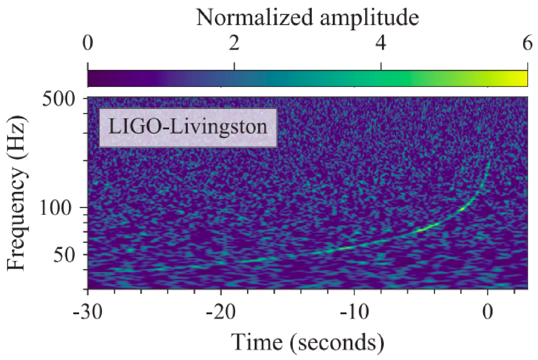
Time–frequency spectrogram labelled LIGO-Livingston: Frequency (Hz) on a logarithmic axis with ticks 50, 100, 500 versus Time (seconds) from -30 to 0; a colour bar of Normalized amplitude from 0 to 6; a bright chirp track rises from about 40 Hz at -20 s to above 100 Hz near 0 s.

1.1 Data from the graph

(1.1.1) You are given semi-logarithmic graph, from which you need to extract values of frequency and time. Let bottom left corner be origin (0,0), horizontal coordinate $x$ is measured in centimeters, find a linear expression to obtain actual time $t$ from $x$ . [2 т.]

(1.1.2) Similarly, find an expression for the frequency $f$ as a function of the vertical coordinate $y$ measured in centimeters. [3 т.]

(1.1.3) Extract 14 values of time and corresponding frequency from the given graph into a table. At least one of the values should correspond to a frequency more than $100\,\mathrm{Hz}$ . [7 т.]

1.2 Calculate system parameters

The most plausible explanation for this evolution of frequency is the in-spiralling of two orbiting masses, $m_1$ and $m_2$ , due to gravitational-wave emission. At the lower frequencies, such evolution is characterized by the “chirp mass”

M_{chirp} = \frac{(m_1 m_2)^{3/5}}{(m_1 + m_2)^{1/5}} = \frac{c^3}{G}\left[\frac{5}{96}\pi^{-8/3} f^{-11/3}\dot{f}\right]^{3/5}

where $f$ and $\dot{f}$ are the observed frequency and its rate of change with respect to time and $G$ and $c$ are the gravitational constant and speed of light.

(1.2.1) From the equation above, derive an expression for the frequency dependence on time.

Note: If $x^n\dot{x} = k$ , then $\frac{x^{n+1}}{(n+1)} = kt + C$ , where $k$ , $n$ and $C$ are constants. [3 т.]

(1.2.2) By plotting the appropriate graph, find the chirp mass and estimate its error caused by uncertainty in slope calculation. [22 т.]

We realise that what is measured by the ground-based GW detectors are actually the detector-frame masses, which are related to the source frame masses by

m_{\mathrm{detector}} = (1+z)m

where $z$ is the redshift of the binary.

(1.2.3) If the host galaxy NGC 4993 has a redshift $z = 0.009783$ , find the source frame chirp mass. [2 т.]

(1.2.4) The mass ratio $q = m_1/m_2$ , is much harder to measure. Advanced waveform analysis shows that $q$ for this system was in the range of 0.73 to 1.0. Calculate range of values for the masses $m_1$ (primary) and $m_2$ (secondary). [6 т.]

Combined original · 1 Data from the graph

Additional original source: Data Analysis Problems & Solutions.pdf. This source has different wording, requests, figures and scoring. Its complete version is retained below; the dated question and matching solution version above stays unchanged. No chronology is printed on this combined source.

Source note. The combined original prints the distance request as 3 points but its key as 2.0. Its uncertainty, sign and mass-subscript discrepancies are retained as printed.

In this problem, we will analyze Time-frequency representations of data containing the gravitational-wave event GW170817, Which was the first observation by LIGO of a merger of a binary neutron star system.

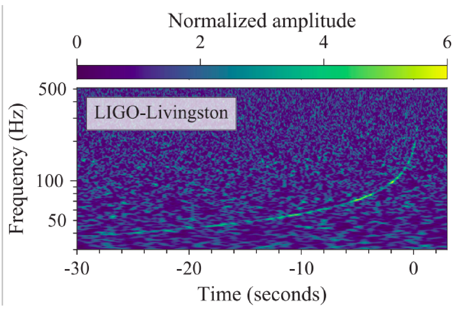
LIGO-Livingston normalized amplitude, frequency and time spectrogram

(1.1) You are given semi-logarithmic graph, from which you need to extract values of frequency and time. Find a linear expression to obtain actual time $t$ from the measured horizontal axis coordinate $x$ . [2 т.]

(1.2) Similarly, find an expression for the frequency $f$ as a function of the measured coordinate $y$ . [3 т.]

(1.3) Using the relations that you obtained, extract at least 12 values of time and corresponding frequency from the given graph. At least one of the values should correspond to a frequency more than 100 Hz. [6 т.]

Combined original · 2 Calculate system parameters

M_{chirp}=\frac{(m_1m_2)^{3/5}}{(m_1+m_2)^{1/5}}=\frac{c^3}{G}\left[\frac5{96}\pi^{-8/3}f^{-11/3}\dot f\right]^{3/5}

where $f$ and $\dot f$ are the observed frequency and its time derivative and $G$ and $c$ are the gravitational constant and speed of light.

(2.1) Linearize the equation given above and obtain the frequency dependence on time.

Note: If $x^n\dot x=k$ , then $\frac{x^{n+1}}{(n+1)}=kt+C$ , where $k$ , $n$ and $C$ are all some constants. [3 т.]

(2.2) Find chirp mass in terms of solar masses and its uncertainty, by using a millimeter paper. [15 т.]

We realise that what is measured by the ground-based GW detectors is actually the detector-frame masses, which are related to the source frame masses by

m_{detector}=(1+z)m

where $z$ is the redshift of the binary.

(2.3) It is known that host galaxy NGC 4993 has a red shift $z=0.009783$ , find the source frame chirp mass. [2 т.]

(2.4) Find distance to the NGC 4993. [3 т.]

(2.5) The mass ratio $q=m_1/m_2$ , is much harder to measure. Advanced waveform analysis shows that $q$ for this system was in the range of 0.73 to 1.0. Calculate range of values for the masses $m_1$ (primary) and $m_2$ (secondary). [6 т.]

Combined original · 3 Speed of the gravitational wave

Gamma-ray burst GRB 170817A was observed by the Fermi Gamma-ray Burst Monitor to be almost simultaneous with gravitational wave event. The same neutron star merger was identified as the source of the signal. In the table below, the first column is time since the arrival of the gravitational wave peak, which happened on 2017 August 17 at 12:41:04 UTC. This peak symbolized the start of the merger of the neutron stars. The second column gives detector counts as measured in Fermi GBM. Background is already subtracted from the signal.

t(s)	event count (/s)
0.5981	15
0.7975	-62
0.9968	9
1.1962	-24
1.3956	24
1.5949	-50
1.7943	0
1.9937	18
2.1930	53
2.3924	179
2.5918	176
2.7911	91
2.9905	26
3.1899	71
3.3892	38
3.5886	59
3.7880	21

(3.1) Plot event count over time on a millimeter paper. [6 т.]

(3.2) Estimate the delay $\Delta t$ between start of the merger and start of the Gamma-ray Burst. [1 т.]

From this measurement it is possible to determine what is called the fractional speed difference during the trip.

\frac{\Delta v}{v_{EM}}=\frac{v_{GW}-v_{EM}}{v_{EM}}

(3.3) Express this quantity in terms of $\Delta t$ and distance to the source $D$ . [1 т.]

(3.4) If we conservatively assume that the peak of the gravitational wave signal and the first GRB photons were emitted simultaneously, thus attributing the entire lag to faster travel by the gravitational wave signal, this time difference provides an upper bound on $\Delta v$ . Calculate this upper bound. [1 т.]

(3.5) To obtain a lower bound on $\Delta v$ , one can assume that the two signals were emitted at times differing by more than $\Delta t$ , with the faster EM signal making up some of the difference. Take maximum time delay as 10s and find lower bound. [1 т.]

Отговори

Решение

1.1 Data from the graph

(1.1.1)

To make the scaling as accurate as possible, we take the time values far apart.

When $x = 0.0\,\mathrm{cm}$ $t = -30\,\mathrm{s}$ , using the ruler we can also measure that at $t = 0\,\mathrm{s}$ we have $x = 10.6\,\mathrm{cm}$ .

For range $\Delta x \geq 10cm$ 1 pt. For $6cm < \Delta x < 10cm$ 0.5 pt. For $3cm < \Delta x < 6cm$ 0.2 pt. For $\Delta x < 3cm$ 0pt.

This leads to

0.0\,\mathrm{cm} = (-30\,\mathrm{s})A + B

10.6\,\mathrm{cm} = (0\,\mathrm{s})A + B = B

A = \frac{10.6\,\mathrm{cm}}{30\,\mathrm{s}} = 0.35\,\mathrm{cm/s} \qquad \mathbf{0.5}

\therefore t = \frac{x - 10.6}{0.35}\mathrm{s} \qquad \mathbf{0.5}

(1.1.2)

Analogues to the previous scaling:

For range $\Delta y \geq 4.5cm$ 1 pt. For $3cm < \Delta y < 4.5cm$ 0.5 pt. For $1.5cm < \Delta y < 3cm$ 0.2 pt. For $y < 1.5cm0pt$ ..

0.0\,\mathrm{cm} = C\log(30\,\mathrm{Hz}) + D

5.3\,\mathrm{cm} = C\log(500\,\mathrm{Hz}) + D \qquad \mathbf{1.0}

5.3\,\mathrm{cm} = C\log\left(\frac{500}{30}\right)

C = 4.34\,\mathrm{cm} \qquad \mathbf{0.25}

D = -6.41\,\mathrm{cm} \qquad \mathbf{0.25}

\therefore f = 10^{\left(\frac{y+6.41}{4.34}\right)}\mathrm{Hz} \qquad \mathbf{0.5}

(1.1.3)

It is not necessary to use $X$ -scaling as students can choose convenient points from the graph.

If has at least one value more that 100Hz 1.4pt.

x(cm)	y(cm)	t(s)	f(Hz)	$f^{-8/3}(Hz^{-8/3})$
-	0.5	-28.0	39.1	5.67E-05
-	0.5	-26.0	39.1	5.67E-05
-	0.6	-24.0	41.3	4.92E-05
-	0.6	-22.0	41.3	4.92E-05
-	0.7	-20.0	43.5	4.27E-05
-	0.8	-18.0	45.9	3.71E-05
-	0.9	-16.0	48.4	3.22E-05
-	1.0	-14.0	51.0	2.79E-05
-	1.1	-12.0	53.8	2.43E-05
-	1.2	-10.0	56.7	2.11E-05
-	1.4	-8.0	63.1	1.59E-05
-	1.6	-6.0	70.1	1.20E-05
-	1.8	-4.0	78.0	0.90E-05
-	2.3	-2.0	101.7	0.43E-05
-	3.4	0.0	182.4	0.09E-05

0.4 points for each row (except last column). Maximum 7 points.

1.2 Calculate system parameters

(1.2.1)

\frac{96}{5}\pi^{8/3}\left(\frac{GM_{chirp}}{c^3}\right)^{5/3} = f^{-11/3}\dot{f} \qquad \mathbf{1.0}

\therefore \left[\frac{96}{5}\pi^{8/3}\left(\frac{GM_{chirp}}{c^3}\right)^{5/3}\right]t + \left[\frac{3}{8}\right]f^{-8/3} + C = 0 \qquad \mathbf{2.0}

(1.2.2)

Calculation of $f^{-8/3}$ for each value 3/14 values 3.0

Graph:

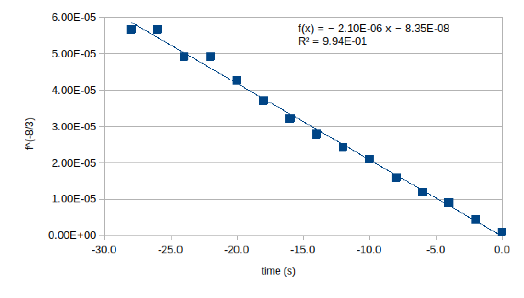
Indicated $X$ axis, written few numbers on the axis and written proper units 1pt. Indicated $Y$ axis, written few numbers on the axis and written proper units 1pt. Used $70-100$ percent of the graphing paper 2pt, for $50-70$ percent 1.5pt, for $30-50$ percent 1pt, for $30-50$ percent 0.5pt. For each correct point (within 2mm distance from the correct positions) on the graph 0.35pt

\mathrm{slope} = -2.10\times 10^{-6} \qquad \mathbf{1.1}

\mathrm{slope} = \frac{8}{3}\left[\frac{96}{5}\pi^{8/3}\left(\frac{GM_{chirp}}{c^3}\right)^{5/3}\right]

M_{chirp} = \left[\left(\frac{5}{256}\right)^{3/5}\frac{c^3}{G}\pi^{-8/5}\right](\mathrm{slope})^{3/5} \qquad \mathbf{2.0}

\therefore M_{chirp} = 2.39\times 10^{30}\,\mathrm{kg} = 1.20M_{\odot} \qquad \mathbf{2.0}

\Delta\mathrm{slope} = 9\times 10^{-8} \qquad \mathbf{2.0}

\frac{\Delta M_{chirp}}{M_{chirp}} = \frac{3}{5}\frac{\Delta\mathrm{slope}}{\mathrm{slope}} = 0.023 \qquad \mathbf{2.0}

\Delta M_{chirp} = 0.03M_{\odot} \qquad \mathbf{1.0}

For uncertainty 70 percent points for the method and 30 percent for the result.

(1.2.3)

M_{chirp} = \frac{M_{chirp_{\mathrm{detactor}}}}{1+z} = \frac{1.20M_{\odot}}{1.009783} = 1.19M_{\odot} \qquad \mathbf{2.0}

(1.2.4)

M_{chirp} = \frac{(m_1 m_2)^{3/5}}{(m_1+m_2)^{1/5}}

\therefore M_{chirp} = m_2\sqrt[5]{\frac{q^3}{1+q}} \qquad \mathbf{2.0}

This is an increasing function of $q$

\therefore m_{2,min} = M_{chirp}2^{1/5} = 1.37M_{\odot}

m_{2,max} = 1.60M_{\odot} \qquad \mathbf{1.0}

Also,

M_{chirp} = \frac{m_1}{q}\sqrt[5]{\frac{q^3}{1+q}} = \frac{m_1}{\sqrt[5]{q^2(1+q)}} \qquad \mathbf{2.0}

\therefore m_{1,max} = M_{chirp}2^{1/5} = 1.37M_{\odot}

m_{2,min} = 1.17M_{\odot} \qquad \mathbf{1.0}

Combined original · 1 Data from the graph

(1.1) To make the scaling as accurate as possible, we take the time values far apart. When $x=0.0\,\mathrm{cm}$ $t=-30\,\mathrm{s}$ , using the ruler we can also measure that at $t=0\,\mathrm{s}$ we have $x=11.1\,\mathrm{cm}$ . 1.0

This leads to

0.0\,\mathrm{cm}=(-30\,\mathrm{s})A+B

11.1\,\mathrm{cm}=(0\,\mathrm{s})A+B=B

A=\frac{11.1\,\mathrm{cm}}{30\,\mathrm{s}}=0.37\,\mathrm{cm/s}

\therefore t=\frac{x-11.1}{0.37}\,\mathrm{s}

1.0

(1.2) Analogues to the previous scaling,

0.0\,\mathrm{cm}=C\log(30\,\mathrm{Hz})+D

5.3\,\mathrm{cm}=C\log(500\,\mathrm{Hz})+D

1.0

5.3\,\mathrm{cm}=C\log\left(\frac{500}{30}\right)

C=4.34\,\mathrm{cm}

D=-6.41\,\mathrm{cm}

\therefore f=10^{\left(\frac{y+6.41}{4.34}\right)}\mathrm{Hz}

2.0

(1.3) It is not necessary to use X-scaling as students can choose convenient points from the graph.

x(cm)	y(cm)	t(s)	f(Hz)	$f^{-8/3}(Hz^{-8/3})$
-	0.5	-28.0	39.1	5.67E-05
-	0.5	-26.0	39.1	5.67E-05
-	0.6	-24.0	41.3	4.92E-05
-	0.6	-22.0	41.3	4.92E-05
-	0.7	-20.0	43.5	4.27E-05
-	0.8	-18.0	45.9	3.71E-05
-	0.9	-16.0	48.4	3.22E-05
-	1.0	-14.0	51.0	2.79E-05
-	1.1	-12.0	53.8	2.43E-05
-	1.2	-10.0	56.7	2.11E-05
-	1.4	-8.0	63.1	1.59E-05
-	1.6	-6.0	70.1	1.20E-05
-	1.8	-4.0	78.0	0.90E-05
-	2.3	-2.0	101.7	0.43E-05
-	3.4	0.0	182.4	0.09E-05

0.5 points for each row (except last column). Maximum 6 points.

Combined original · 2 Calculate system parameters

(2.1)

\frac{96}{5}\pi^{8/3}\left(\frac{GM_{chirp}}{c^3}\right)^{5/3}=f^{-11/3}\dot f

\therefore\left[\frac{96}{5}\pi^{8/3}\left(\frac{GM_{chirp}}{c^3}\right)^{5/3}\right]t+\left[\frac38\right]f^{-8/3}+C=0

3.0

(2.2)

Original plotted f^(-8/3) against time and printed fit

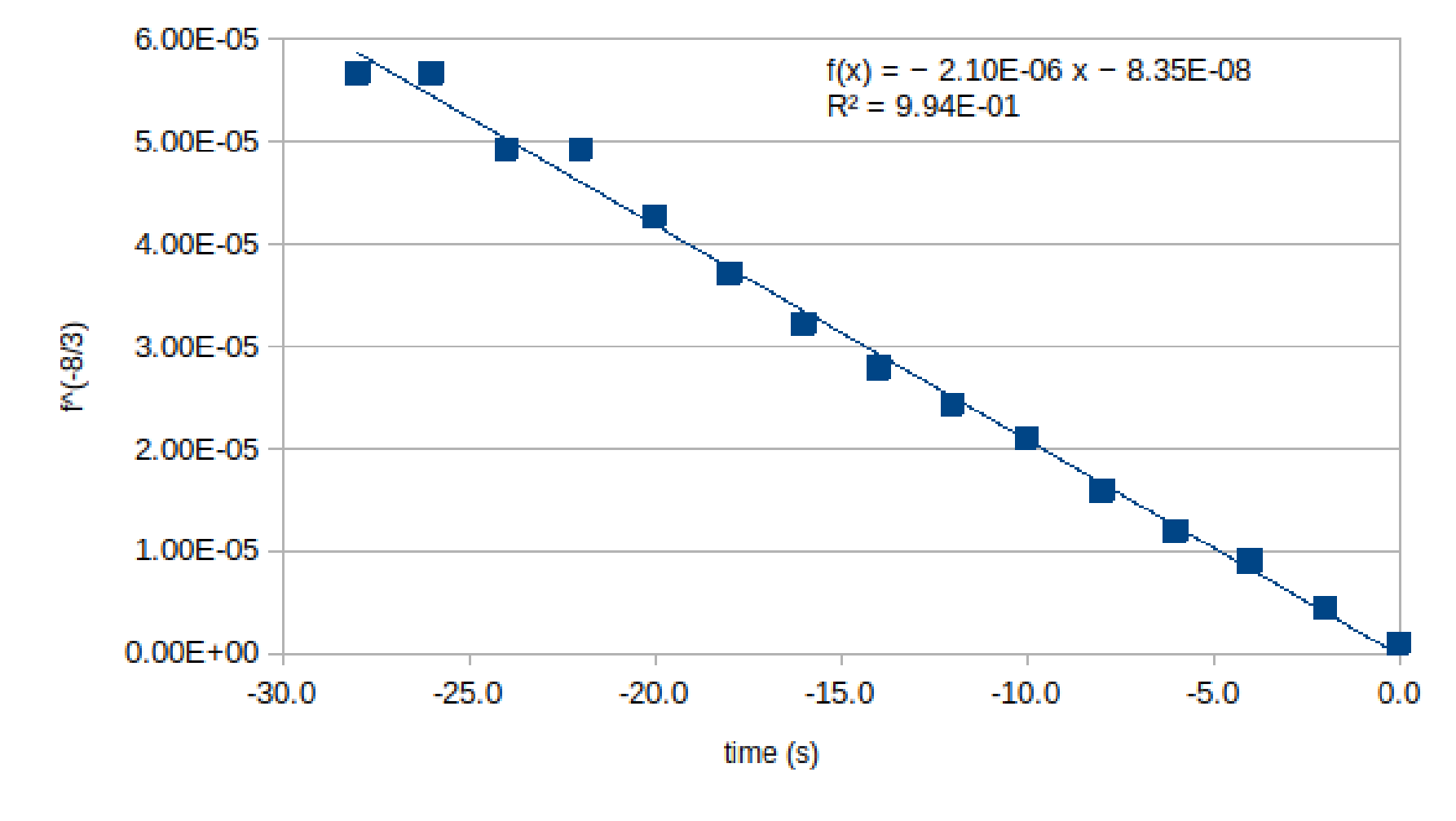
Calculation of $f^{-8/3}$ values 3.0

Properly drawn graph 6.0

\mathrm{slope}=\frac83\left[\frac{96}{5}\pi^{8/3}\left(\frac{GM_{chirp}}{c^3}\right)^{5/3}\right]

M_{chirp}=\left[\left(\frac5{256}\right)^{3/5}\frac{c^3}{G}\pi^{-8/5}\right](\mathrm{slope})^{3/5}

2.0

\mathrm{slope}=2.10\times10^{-6}

2.0

\therefore M_{chirp}=2.39\times10^{30}\,\mathrm{kg}=1.20M_\odot

2.0

with 95% confidence interval

\Delta\mathrm{slope}=9\times10^{-8}

\frac{\Delta M_{chirp}}{M_{chirp}}=\frac35\frac{\Delta\mathrm{slope}}{\mathrm{slope}}=0.04

\Delta M_{chirp}=0.03M_\odot

(2.3)

M_{chirp}=\frac{M_{chirp_{detactor}}}{1+z}=\frac{1.20M_\odot}{1.009783}=1.19M_\odot

2.0

(2.4) According to the Hubble law,

D=\frac{zc}{H}=\frac{0.009783\times3\times10^5}{70}=41.9\,\mathrm{Mpc}

2.0

(2.5)

M_{chirp}=\frac{(m_1m_2)^{3/5}}{(m_1+m_2)^{1/5}}

\therefore M_{chirp}=m_2\sqrt[5]{\frac{q^3}{1+q}}

2.0

This is an increasing function of $q$

\therefore m_{2,min}=M_{chirp}2^{1/5}=1.37M_\odot

m_{2,max}=1.60M_\odot

1.0

\mathrm{Also},\ M_{chirp}=\frac{m_1}{q}\sqrt[5]{\frac{q^3}{1+q}}=\frac{m_1}{\sqrt[5]{q^2(1+q)}}

2.0

\therefore m_{1,max}=M_{chirp}2^{1/5}=1.37M_\odot

m_{2,min}=1.17M_\odot

1.0

Combined original · 3 Speed of the gravitational wave

(3.1)

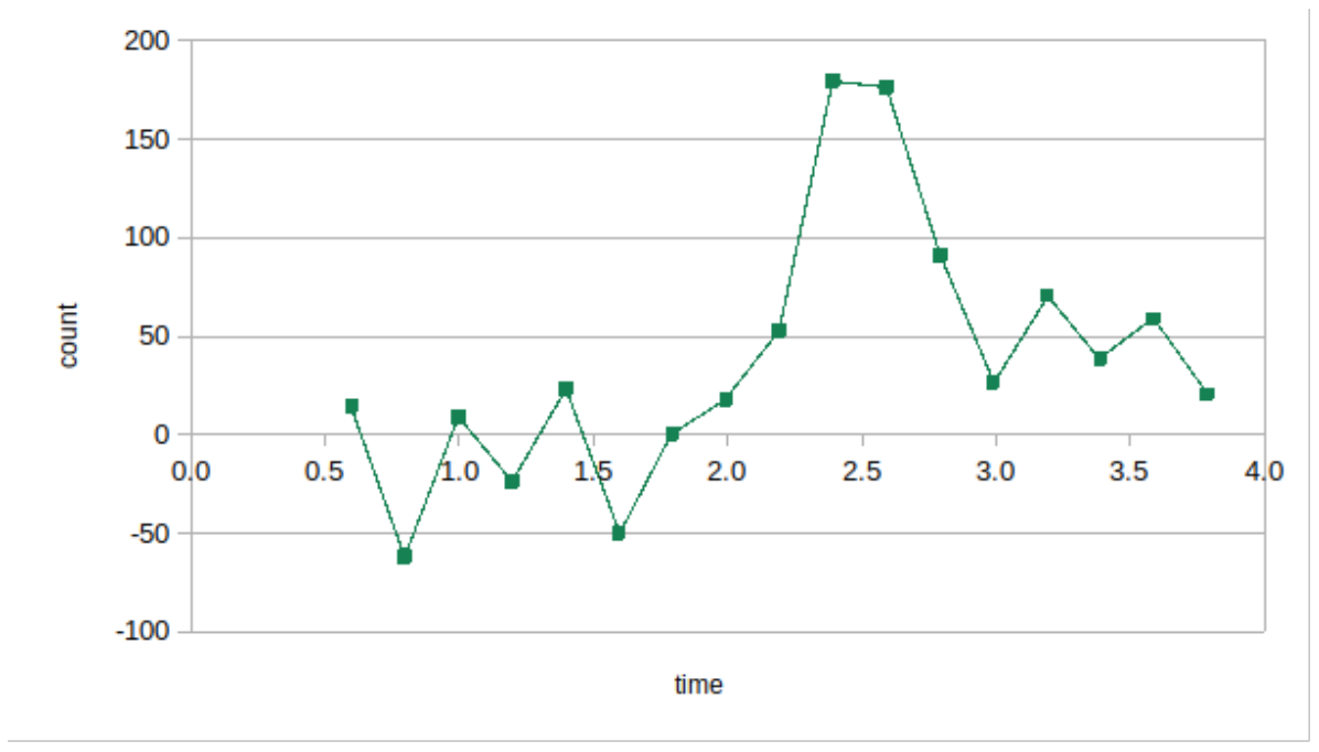
(3.2) It appears that the event is starting from $\Delta t=1.8\,\mathrm{s}$ . Some students may also write $\Delta t=2.2\,\mathrm{s}$ as that is when the signal is truly above fluctuations seen before the event. We will accept both the answers. 1.0

(3.3) By simple substitution we can calculate that

\frac{\Delta v}{v_{EM}}=\frac{\Delta t v_{GW}}{D}\approx\frac{\Delta tc}{D}

1.0

(3.4)

\frac{\Delta v}{v_{EM}}=4.2\times10^{-16}\ \mathrm{to}\ 5.1\times10^{-16}

1.0

(3.5)

\Delta t'=\Delta t-10=-8.2\,\mathrm{s}\ \mathrm{to}\ 7.8\,\mathrm{s}

From this time delay

\frac{\Delta v}{v_{EM}}=-1.9\times10^{-15}\ \mathrm{to}\ 1.8\times10^{-15}

1.0

Оригинал в Архива: IOAA-Data.pdf · официални решения: Data_Solution.pdf · допълнителни данни: Data Analysis Problems & Solutions.pdf