Съдържание

Условие Stellar parameters Radial Velocity method Transit method (without limb darkening)Introducing limb darkening Transit in the presence of limb darkening Решение

IOAA 2025, Анализ на данни — Задача 1. D01 · 30 Years of Exoplanets

Оригинал на условието (PDF)Съобщи за грешка

Всички материали от IOAA 2025

18th IOAA, Mumbai 2025 — Data Analysis Examination · 90 т.

Внимание: Бележка към темата

The obtained Summary Answersheet contains D02 only. Referenced D01 response forms were unavailable; all D01 data graphs printed in the question and solution booklets are retained.

Условие

This problem explores some aspects of the two main methods of exoplanet detection: radial velocity and transit. Throughout this problem we shall consider a particular system of a single planet (P) in a circular orbit with radius $a$ around a solar-type star (S). We shall refer to this system as the “SP system”.

Stellar parameters

(D01.1) [8 marks] The V-band apparent magnitude of the star S is $(7.65\pm0.03)\ \mathrm{mag}$ , the parallax is $(20.67\pm0.05)$ milliarcsecond and the bolometric correction (BC) is $-0.0650\ \mathrm{mag}$ . Thus the star has a higher bolometric luminosity than its luminosity in the V-band.

Estimate the mass of the star, $M_s$ (in units of $M_\odot$ ), assuming a mass-luminosity ( $M$ – $L$ ) relation of the form $L\propto M^4$ . Also estimate the uncertainty in $M_s$ . You may need $\frac d{dx}\ln x=\frac1x$ .

Radial Velocity method

The radial velocity method uses the Doppler shift $\delta\lambda\equiv\lambda_{\mathrm{obs}}-\lambda_0$ between the observed wavelength $\lambda_{\mathrm{obs}}$ and the rest wavelength $\lambda_0$ of a known spectral line to detect an exoplanet and determine its characteristics.

The figure below shows the $\delta\lambda$ for the Fe I line $(\lambda_0=543.45\times10^{-9}\ \mathrm{m})$ as a function of time as observed for the SP system.

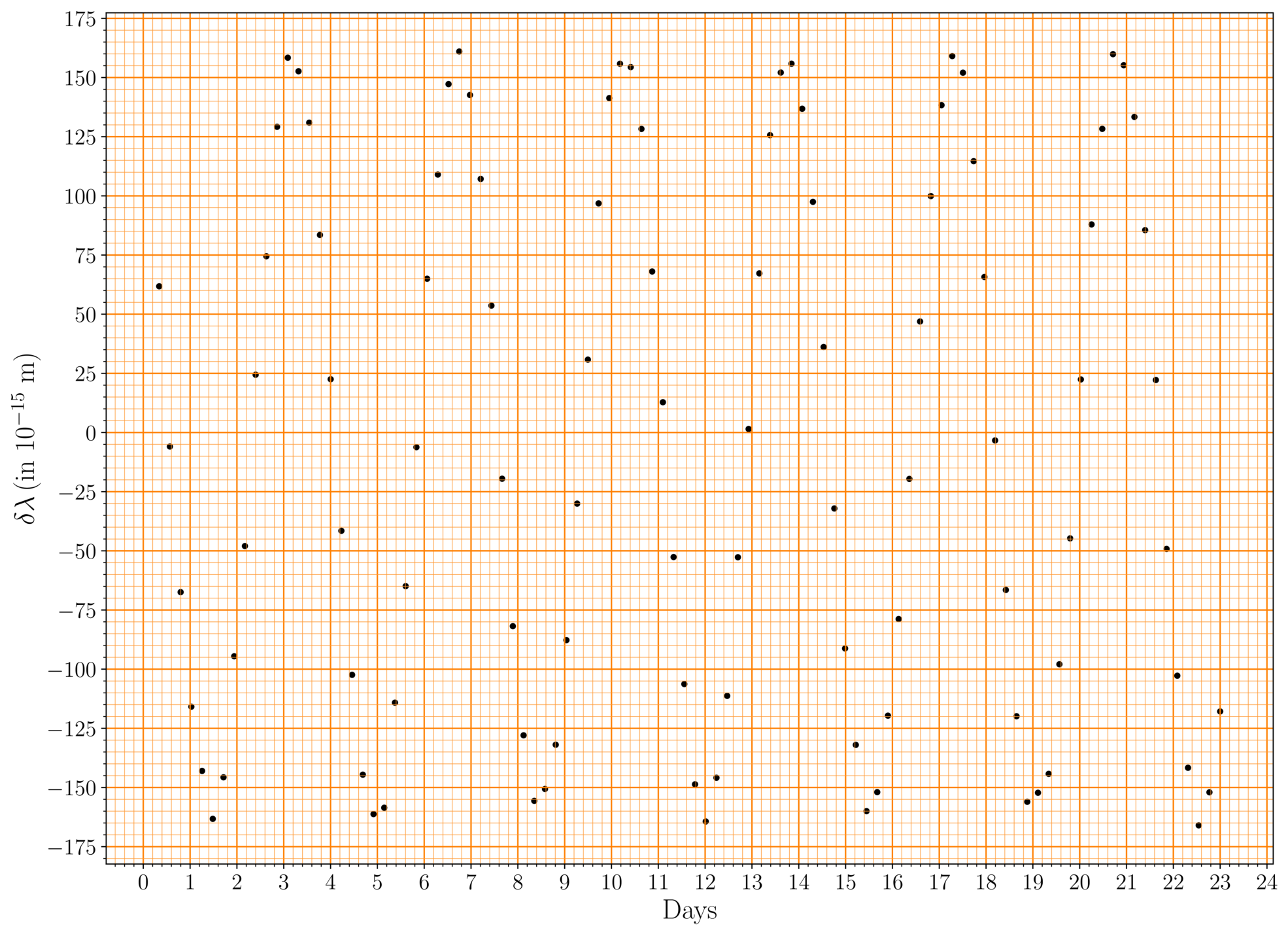
Original observed Fe I wavelength-shift data, every point, full grid, wavelength axis and Days axis.

The radial velocity semi-amplitude $K$ is defined as $K\equiv(v_{r,\max}-v_{r,\min})/2$ where $v_{r,\max}$ and $v_{r,\min}$ are the minimum and maximum radial velocities, respectively. For a circular planetary orbit the semi-amplitude $K$ can be written as:

K=\left(\frac{2\pi G}T\right)^{1/3}\frac{M_p\sin i}{(M_p+M_s)^{2/3}}

where $T$ is the period, $i$ is the inclination of the planetary orbit (angle between the normal to the orbital plane of the planet and the line of sight of the observer), $M_p$ and $M_s$ are the masses of the planet and the star, respectively.

(D01.2) Use the graph given in the Summary Answersheet to answer the following.

(D01.2a) [2 marks] Draw a smooth curve associated with the observed data shown in the graph.

(D01.2b) [11 marks] Select appropriate points on your drawn curve and use suitable methods to determine $T$ and $K$ along with respective uncertainties. All data points used for the calculation of $T$ and $K$ must be shown in the table in the Summary Answersheet. Use the rest of the table to show your intermediate calculations, as needed, with appropriate headers.

(D01.2c) [5 marks] Find the minimum mass of the planet $M_{p,\min}$ (in $M_\odot$ ), and its corresponding uncertainty, assuming $M_p\ll M_s$ .

(D01.2d) [4 marks] Using the value of $M_{p,\min}$ estimated in part (D01.2c), calculate the minimum value of the semi-major axis of the planet’s orbit, $a_{\min}$ , in au and its uncertainty.

Transit method (without limb darkening)

The schematic diagram of a planet transit (not drawn to scale) is shown below. Initially, we shall assume the stellar disk to have a uniform average intensity with some intrinsic noise due to the star itself.

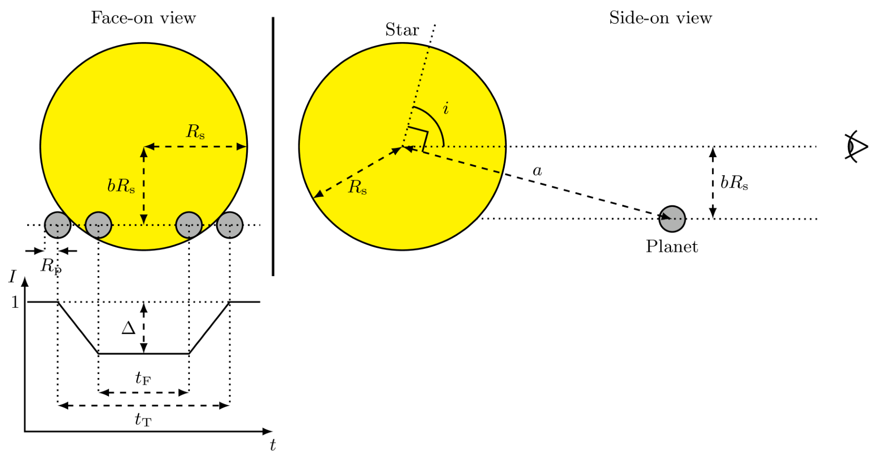
Original face-on and side-on transit geometry and full schematic lightcurve: all planet positions, radii, b, i, a, observer, Delta, tT and tF.

The lightcurve of the normalized intensity, $I$ , as a function of time $t$ is shown in the schematic diagram of the transit above. The average stellar intensity outside the transit is taken as unity. The maximum decrease in the intensity is given by $\Delta$ in the normalized light curve. For a uniformly bright stellar disk, the radius of the planet, $R_p$ , is related to $\Delta$ as

\left(\frac{R_p}{R_s}\right)^2=\Delta,

where $R_s$ is the radius of the star.

The total duration of transit (when part or all of the planet covers the stellar disk) is given by $t_T$ , while $t_F$ gives the duration when the planet is fully in front of the stellar disk. The “impact parameter” $b$ is the projected distance between the planet and centre of the stellar disk at the mid-point of the transit, in units of the stellar radius, $R_s$ .

For a nearly edge-on star-planet orbit, the impact parameter is given by the formula

b=\left[\frac{(1-\sqrt\Delta)^2-(t_F/t_T)^2(1+\sqrt\Delta)^2}{1-(t_F/t_T)^2}\right]^{1/2}

(D01.3) [3 marks] For the SP system, the stellar radius is known to be $R_s=1.20\,R_\odot$ , and the transit of the planet is indeed visible. Using the minimum orbital radius, $a_{\min}$ , estimated in part (D01.2d), find the minimum value, $i_{\min}$ , of the inclination angle.

Assuming a stellar disk of uniform brightness, the transit lightcurve would look like as shown below.

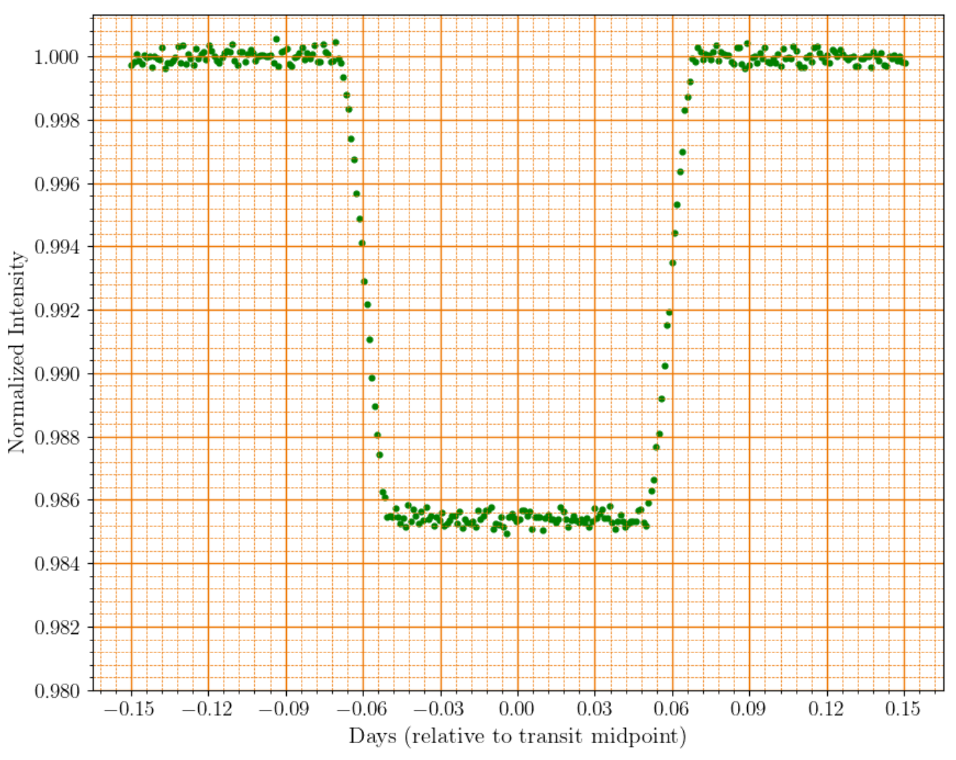
Original measured transit lightcurve, normalized-intensity and time axes, complete grid and data points.

(D01.4) Using the given lightcurve answer the following questions. For your reference the above lightcurve is also given in the Summary Answersheet.

(D01.4a) [3 marks] Estimate the values of $t_T$ and $t_F$ in days by marking appropriate readings on the graph.

(D01.4b) [2 marks] Estimate the mean value of $\Delta$ , by marking appropriate readings on the graph and hence find $R_p$ in units of $R_\odot$ .

(D01.4c) [2 marks] Determine the value of $i$ in degrees assuming the orbital radius to be $a_{\min}$ .

Introducing limb darkening

So far we have assumed the stellar disk to be uniformly bright. In reality, the observed brightness of the stellar disk is not uniform due to “limb darkening” — an optical effect where the central part of the stellar disk appears brighter than the edge, or the “limb”.

The limb darkening effect can be measured by the relative intensity $J(\theta)\equiv\frac{I(\theta)}{I(0)}$ , where $\theta$ is the angle between the normal to the stellar surface at a point and the line joining the observer to that point, $I(\theta)$ is the observed intensity of the stellar disk at that point ( $I(0)$ being the intensity at the centre of the stellar disk). For a distant observer, $\theta$ varies from $\theta=0$ (centre of the disk) to $\theta\approx90^\circ$ (edge of the disk).

(D01.5) The table below gives measured $J(\theta)$ at a certain wavelength for the Sun. We shall assume that the same limb darkening profile holds for the star S.

$\theta$	$J(\theta)$	$\theta$	$J(\theta)$	$\theta$	$J(\theta)$	$\theta$	$J(\theta)$
$0^\circ$	1.000	$20^\circ$	0.971	$40^\circ$	0.883	$70^\circ$	0.595
$10^\circ$	0.994	$25^\circ$	0.950	$50^\circ$	0.794	$80^\circ$	0.475
$15^\circ$	0.984	$30^\circ$	0.943	$60^\circ$	0.724	$90^\circ$	0.312

The limb darkening profile can be modelled by a quadratic formula:

J(\theta)=1-a_1(1-\cos\theta)-a_2(1-\cos\theta)^2,

where $a_1$ and $a_2$ are two constants.

We shall estimate the unknown coefficients $a_1$ and $a_2$ from the given data by making a plot with suitable variables.

(D01.5a) [2 marks] Choose a pair of variables $(x_1,y_1)$ which are suitable functions of $\theta$ and $J$ , that you want to plot along $x$ and $y$ axes, respectively, to determine $a_1$ and $a_2$ . Write the expressions for $x_1$ and $y_1$ .

If you need to define additional variables for additional plots, define them as $(x_2,y_2)$ , etc.

(D01.5b) [4 marks] Tabulate the values necessary for your plots.

(D01.5c) [7 marks] Plot the newly defined variables on the given graph paper (mark your graph as “D01.5c”).

(D01.5d) [7 marks] Obtain $a_1$ and $a_2$ from the plot. Uncertainties on the values are not needed.

Transit in the presence of limb darkening

Now, we consider planetary transits across a limb darkened stellar disk. In the presence of limb darkening, which we shall model by the quadratic formula of $J(\theta)$ given above, the average observed intensity of the entire stellar disk (without any transit), $\langle I\rangle$ , is given by:

\langle I\rangle=\left(1-\frac{a_1}3-\frac{a_2}6\right)I(0)

Further, the dip in the light caused by the transiting planet now depends not only on the relative size of the planet and the star, $\left(\frac{R_p}{R_s}\right)$ , but also on the intensity profile of the stellar disk along the transit chord, which in turn, depends on the angle of inclination, $i$ .

The schematic diagram below (not drawn to scale) shows the configuration. Note that the brighter part of the star is shown in a darker shade, while the planet is shown as a black dot.

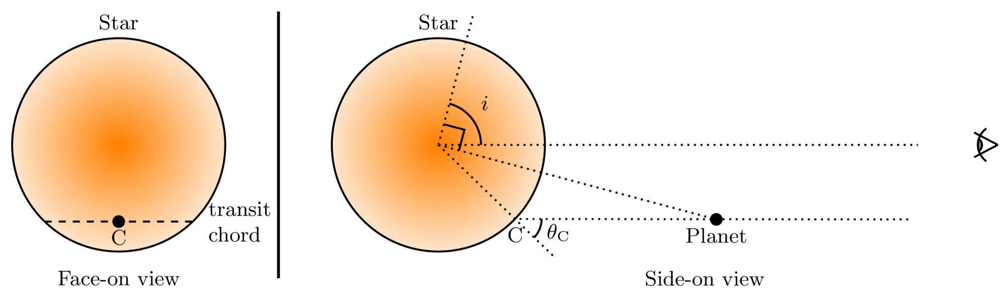
Original limb-darkened stellar transit face-on and side-on views, transit chord, C, i, thetaC, planet and observer.

Here the relation between $\left(\frac{R_p}{R_s}\right)$ and the measured $\Delta$ from the light curve is

\Delta=\frac{I(\theta_C)}{\langle I\rangle}\left(\frac{R_p}{R_s}\right)^2,

where $I(\theta_C)$ is the intensity of the stellar disk at the midpoint of the transit chord (point C in the figure above), $\theta_C$ being the angle between the line of sight and the normal to the surface at that point. From the above it is obvious that for a given star, the same value of $\Delta$ can be produced by many combinations of the planet size, $R_p$ , and the inclination angle $i$ .

(D01.6) It is possible to uniquely determine both $R_p$ and $i$ by using data from transit lightcurves at two wavelengths, say, $\lambda_B$ (blue) and $\lambda_R$ (red). The limb darkening coefficients for these two wavelengths are given below:

Wavelength	$a_1$	$a_2$
$\lambda_B$	0.82	0.05
$\lambda_R$	0.24	0.20

(D01.6a) [2 marks] Choose the correct statement among the following that describes the relation between the maximum depth of the transit ( $\Delta$ ) for $\lambda_B$ and the inclination angle ( $i$ ) of the orbit and tick (✓) it in the Summary Answersheet.

(A) $\Delta$ increases with decreasing $i$ .

(B) $\Delta$ decreases with decreasing $i$ .

(D01.6b) [4 marks] The maximum depth of the transit ( $\Delta$ ) for the “SP system” was measured to be 0.0182 and 0.0159 for $\lambda_B$ and $\lambda_R$ , respectively.

Draw schematic transit light curves for both $\lambda_B$ and $\lambda_R$ on the given grid and label the curves by “B” and “R” respectively. Assume that the total transit duration is same for both wavelengths. The curves need not be to scale, but should represent the shapes of the light curves correctly.

(D01.7) We shall use a graphical method to find the values of $R_p$ and $i$ for the SP system using measurements of $\Delta$ at $\lambda_B$ and $\lambda_R$ .

(D01.7a) [6 marks] Write an appropriate expression connecting the relevant variables that are to be plotted. (Hint: You may consider $i$ or $b$ , and $R_p$ among the relevant variables.)

(D01.7b) [5 marks] Tabulate the appropriate quantities that are to be plotted.

(D01.7c) [7 marks] Draw a suitable graph and mark it as “D01.7c”.

(D01.7d) [4 marks] Estimate the values of $R_p$ (in $R_\odot$ ) and $i$ (in degrees) from the graph.

(D01.8) [2 marks] Based on the results obtained in this problem, indicate whether the planet P is “ROCKY” or “GASEOUS” by ticking (✓) the appropriate box in the Summary Answersheet.

Решение

(D01.1) Solution:

Given

Parallax: $p=(20.67\pm0.05)$ milliarcsecond

V-band apparent magnitude: $m_V=(7.65\pm0.03)\ \mathrm{mag}$

Let:

V-band absolute magnitude: $M_V$

Bolometric Magnitude: $M_{\mathrm{bol}}$

Bolometric Magnitude of the Sun: $M_{\mathrm{bol},\odot}=4.74\ \mathrm{mag}$ (given)

\begin{aligned}M_V&=m_V+5(\log p+1)=4.227\ \mathrm{mag}\\M_{\mathrm{bol}}&=M_V+BC\\&=m_V+5(\log p+1)+BC=4.162\ \mathrm{mag}\end{aligned}

Also $M_{\mathrm{bol}}=M_{\mathrm{bol},\odot}-2.5\log\frac{L_{\mathrm{bol}}}{L_\odot}$

\therefore\quad L_{\mathrm{bol}}=10^{\frac{M_{\mathrm{bol},\odot}-M_{\mathrm{bol}}}{2.5}}L_\odot=6.521\times10^{26}\ \mathrm W

Then $M_s=\left(\frac{L_{\mathrm{bol}}}{L_\odot}\right)^{1/4}M_\odot=1.14\,M_\odot$

Uncertainty estimate:

\begin{aligned}\Delta M_{\mathrm{bol}}&=\sqrt{(\Delta m_V)^2+\left(\frac5{\ln10}\frac{\Delta p}p\right)^2}\\&=0.03\ \mathrm{mag}\end{aligned}

Now, $M_s=10^{\frac{M_{\mathrm{bol},\odot}-M_{\mathrm{bol}}}{10}}$

\begin{aligned}\therefore\quad\Delta M_s&=M_s\frac{\Delta M_{\mathrm{bol}}}{10}\ln10\\&=0.01\,M_\odot\end{aligned}

\boxed{M_s=(1.14\pm0.01)\,M_\odot}

(D01.2a) Solution:

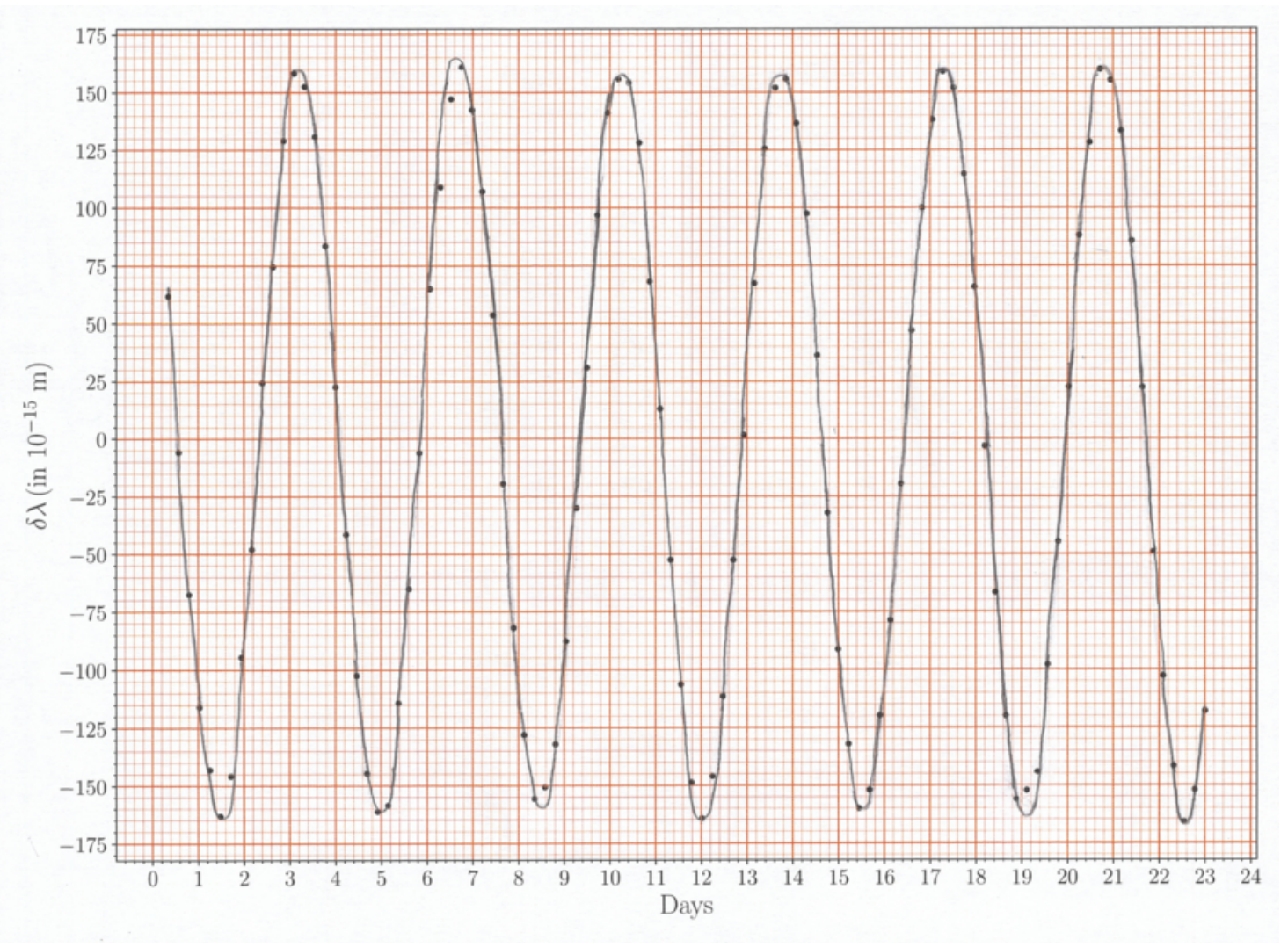
Original official smooth radial-velocity fit with all original data points, grid, axes and periods.

(D01.2b) Solution:

$T$ Determination:

Least count on time axis $=0.2\ \mathrm d$

There are 13 zero crossings (ZC) and 6 periods.

Difference between ZC-1 and ZC-13 $=(21.6-0.6)=21.0\ \mathrm d$

T=\frac{21}6=3.5\ \mathrm d

Uncertainty in $T$ :

\Delta T=\frac16\sqrt{(0.2^2+0.2^2)}=0.05\ \mathrm d

\boxed{T=(3.50\pm0.05)\ \mathrm d}

$K$ Determination:

Serial No. of Extrema	Values of Extrema ( $\times10^{-15}\ \mathrm m$ )	$2\delta\lambda$ m
1	−165
2	160	325
3	−160
4	165	325
5	−160
6	155	315
7	−165
8	155	320
9	−160
10	160	320
11	−165

Least count on $\delta\lambda$ axis $=5\times10^{-15}\ \mathrm m$

Differences in measured extrema ( $\delta\lambda$ ) of alternate pairs are written in table.

\begin{aligned}2(\delta\lambda)_{\mathrm{Mean}}&=321.67\times10^{-15}\ \mathrm m\\(\delta\lambda)_{\mathrm{Mean}}&=160.83\times10^{-15}\ \mathrm m\\K&=\frac{\delta\lambda}\lambda\times c\\&=\frac{160.83\times10^{-15}\times2.998\times10^8}{543.45\times10^{-9}}\\&=88.73\ \mathrm{m\ s^{-1}}\end{aligned}

Uncertainty in $K$ :

\begin{aligned}\sigma_{\delta\lambda}&=\sqrt{\frac1{N-1}\Sigma\left(\delta\lambda-(\delta\lambda)_{\mathrm{Mean}}\right)^2}\\&=2.041\times10^{-15}\ \mathrm m\\\sigma_K&=\frac{\sigma_{\delta\lambda}}\lambda\times c\\&=\frac{2.041\times10^{-15}\times2.998\times10^8}{543.45\times10^{-9}}=1.12\ \mathrm{m\ s^{-1}}\end{aligned}

\boxed{K=(89\pm1)\ \mathrm{m\ s^{-1}}}

(D01.2c) Solution:

The minimum mass of the planet $M_{p,\min}\equiv M_p\sin i$ comes from equation of $K$ .

K=\left(\frac{2\pi G}T\right)^{1/3}\frac{M_p\sin i}{(M_p+M_s)^{2/3}}

We assume $M_p+M_s\approx M_s$ .

For $M_s=1.14\,M_\odot$ , $T=3.5\ \mathrm d$ :

M_{p,\min}\approx KM_s^{2/3}\left(\frac T{2\pi G}\right)^{1/3}=6.927\times10^{-4}\,M_\odot

Uncertainty in $M_{p,\min}$ :

\begin{aligned}\Delta M_{p,\min}&=M_{p,\min}\sqrt{\left(\frac{\Delta K}K\right)^2+\left(\frac23\frac{\Delta M_s}{M_s}\right)^2+\left(\frac13\frac{\Delta T}T\right)^2}\\&=0.091\times10^{-4}\,M_\odot\end{aligned}

\boxed{M_{p,\min}=(6.93\pm0.09)\times10^{-4}\,M_\odot}

(D01.2d) Solution:

\begin{aligned}a_{\min}&=\left(\frac{T^2G(M_s+M_p\sin i)}{4\pi^2}\right)^{1/3}=\left(\frac{T^2G(M_s+M_{p,\min})}{4\pi^2}\right)^{1/3}\\&=0.0471\ \mathrm{au}\end{aligned}

Uncertainty in $a_{\min}$ :

\begin{aligned}\Delta a_{\min}&=a_{\min}\sqrt{\left(\frac23\frac{\Delta T}T\right)^2+\left(\frac13\right)^2\frac{(\Delta M_s)^2+(\Delta M_{p,\min})^2}{(M_s+M_{p,\min})^2}}\\&=0.0005\ \mathrm{au}\end{aligned}

\boxed{a_{\min}=(0.0471\pm0.0005)\ \mathrm{au}}

(D01.3) Solution:

bR_s=a\cos i\qquad\Longrightarrow\quad i=\cos^{-1}\frac{bR_s}a

The minimum value of $i$ corresponds to the maximum value of $b(=1)$ and the minimum value of $a$ . Therefore,

i_{\min}=\cos^{-1}\left(\frac{b_{\max}R_s}{a_{\min}}\right)=\cos^{-1}\left(\frac{R_s}{a_{\min}}\right)=\cos^{-1}\left(\frac{1.20\,R_\odot}{0.0471\ \mathrm{au}}\right)

\boxed{i_{\min}=83.20^\circ}

(D01.4a) Solution:

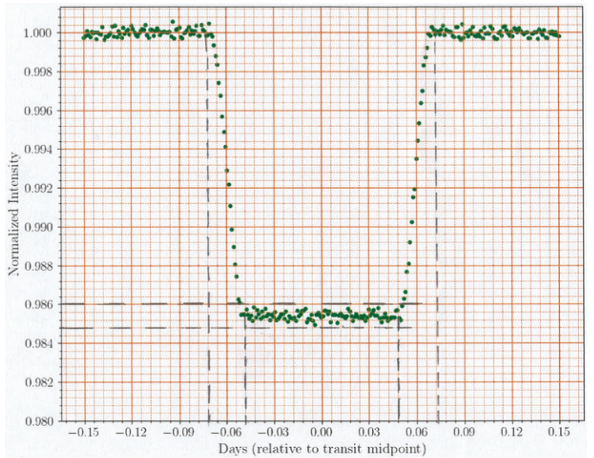
Original official transit-lightcurve readings and annotations, full data, grid and both axes.

In the figure of the transit curve, least count on time axis $=0.006\ \mathrm d$ , and on the intensity axis $=4\times10^{-4}$ .

The measurements on the left and right edges of the transit for $t_T$ are $-0.072\ \mathrm d$ and $0.072\ \mathrm d$ .

The measurements on the left and right edges of the transit for $t_F$ are $-0.048\ \mathrm d$ and $0.048\ \mathrm d$ .

Therefore,

\boxed{t_T=0.144\ \mathrm d}

\boxed{t_F=0.096\ \mathrm d}

(D01.4b) Solution:

The value of the dip is $(0.9860+0.9848)/2=0.9854$

$\Delta$ measured from the graph is $1-0.9854=0.0146$

\therefore\quad\frac{R_p}{R_s}=\sqrt\Delta=0.121

\Longrightarrow\quad R_p=0.121R_s

\boxed{R_p=0.145\,R_\odot}

(D01.4c) Solution:

b=\left[\frac{(1-\sqrt\Delta)^2-(t_F/t_T)^2(1+\sqrt\Delta)^2}{1-(t_F/t_T)^2}\right]^{1/2}

Plugging in values of $\Delta$ , $t_T$ , and $t_F$ , we get $b=0.622$

bR_s=a\cos i

Putting $a=a_{\min}$ ,

\begin{aligned}i&=\cos^{-1}\left(\frac{bR_s}{a_{\min}}\right)\\&=\cos^{-1}\left(\frac{0.622\times1.2\,R_\odot}{0.0471\ \mathrm{au}}\right)\end{aligned}

\boxed{i=85.77^\circ}

(D01.5a) Solution:

Define $\boxed{x_1=1-\cos\theta}$ and $\boxed{y_1=\frac{J-1}{1-\cos\theta}\equiv\frac{J-1}{x_1}}$

Then, $y_1=-a_1-a_2x_1$

In this method $a_1$ and $a_2$ can be determined from the intercept and slope, respectively, of a best fit straight line to a plot of $y_1$ vs $x_1$ .

(D01.5b) Solution:

$\theta$	$J(\theta)$	$x_1$	$y_1$
$0^\circ$	1.000	0.000	×
$10^\circ$	0.994	0.015	−0.395
$15^\circ$	0.984	0.034	−0.470
$20^\circ$	0.971	0.060	−0.481
$20^\circ$	0.970	0.060	−0.497
$25^\circ$	0.950	0.094	−0.534
$30^\circ$	0.943	0.134	−0.425
$40^\circ$	0.883	0.234	−0.500
$40^\circ$	0.890	0.234	−0.470
$50^\circ$	0.794	0.357	−0.577
$60^\circ$	0.724	0.500	−0.552
$70^\circ$	0.595	0.658	−0.616
$80^\circ$	0.475	0.826	−0.635
$90^\circ$	0.312	1.000	−0.688

(D01.5c) Solution:

Plot of $y_1$ vs $x_1$ with straight line fit:

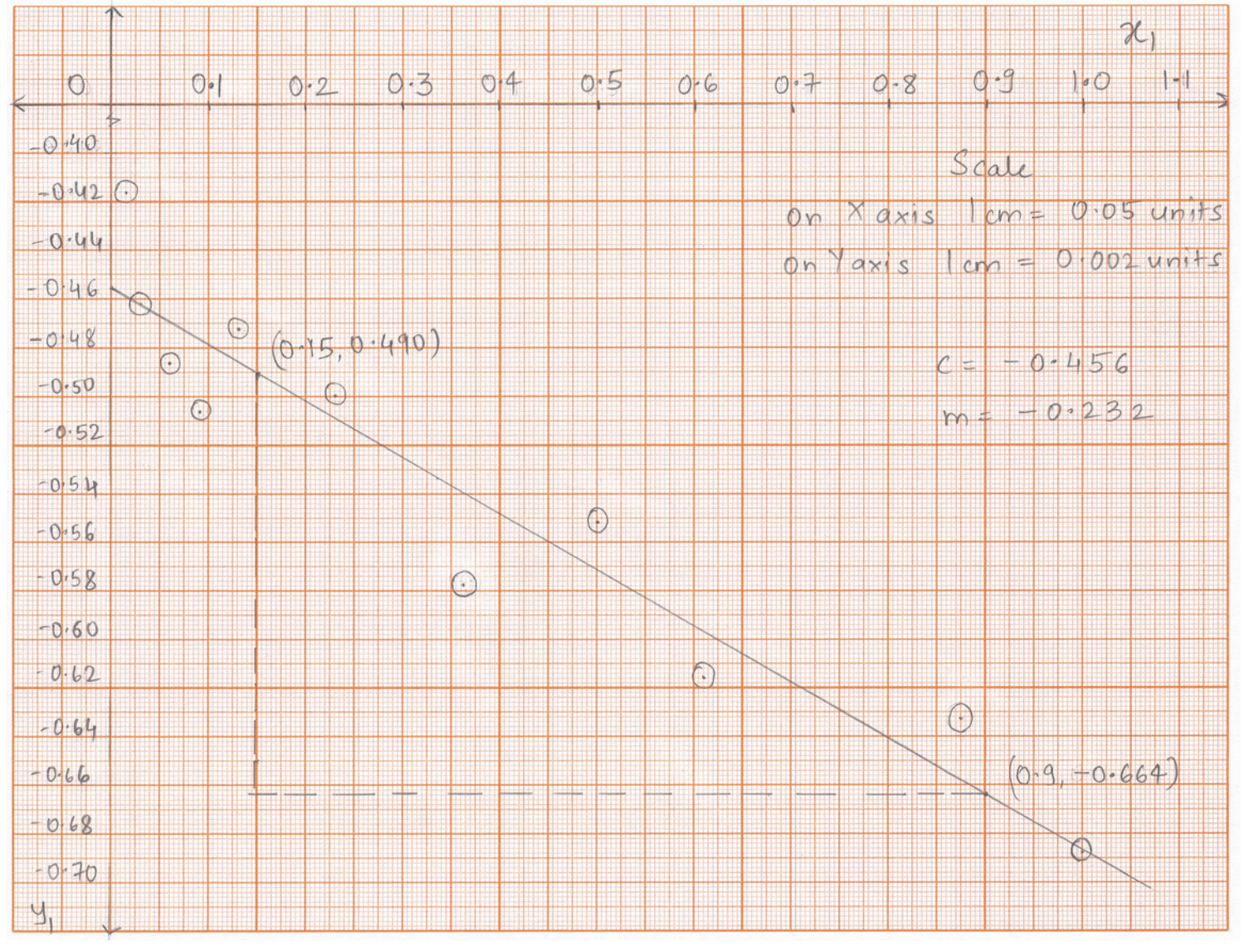
Original official hand-plotted limb-darkening linear fit, all points, scales, slope/intercept and coordinates.

(D01.5d) Solution:

Slope of best fit line $=-0.232$ ; Intercept $=-0.456$

\boxed{\Longrightarrow\quad a_1=0.46,\quad a_2=0.23}

(D01.6a) Solution:

As $i$ decreases, the transit chord moves closer to the limb and the contribution of the midpoint of the transit to the dip in the average brightness reduces. Therefore, $\Delta$ decreases with decreasing $i$ .

Correct option: B

(D01.6b) Solution:

Since the limb darkening effect is stronger for $\lambda_B$ , it causes lesser reduction in the total light at the ingress and egress and more reduction at the transit centre, than for $\lambda_R$ . Therefore, the curves must intersect.

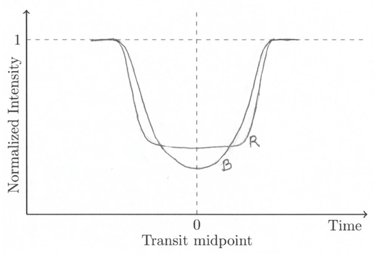
Original official B and R transit lightcurve sketch, both intersecting curves, axes, normalized intensity, time and transit midpoint.

(D01.7a) Solution:

\Delta=\frac{I(\theta_C)}{\langle I\rangle}\left(\frac{R_p}{R_s}\right)^2

\Longrightarrow\quad\left(\frac{R_p}{R_s}\right)^2=\frac{\Delta\langle I\rangle}{I(\theta_C)}

Here, $I(\theta_C)$ is a function of $i$ . Further, $\langle I\rangle=(1-a_1/3-a_2/6)I(0)$ .

Original official stellar chord triangle: full star circle, normal, thetaC, i, Rs, bRs, a, C and planet.

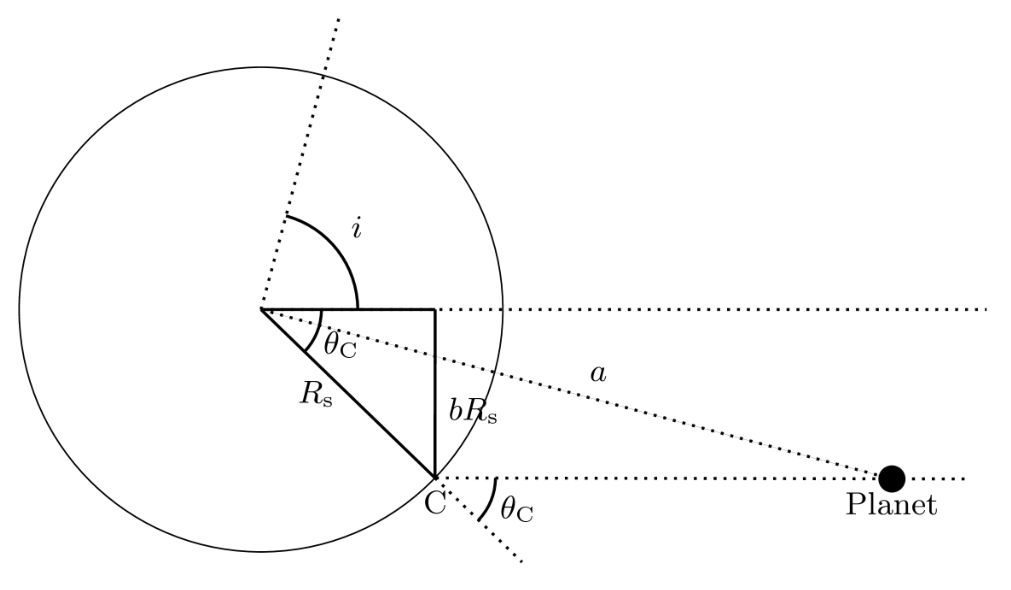
From the figure,

\sin\theta_C=\frac{bR_s}{R_s}=b=\frac{a\cos i}{R_s}

\Longrightarrow\quad\cos\theta_C=\sqrt{1-b^2}=\sqrt{1-\left(\frac{a\cos i}{R_s}\right)^2}

Therefore,

\begin{aligned}I(\theta_C)&=J(\theta_C)I(0)\\&=\left[1-a_1(1-\cos\theta_C)-a_2(1-\cos\theta_C)^2\right]I(0)\\&=\left[1-a_1\left(1-\sqrt{1-b^2}\right)-a_2\left(1-\sqrt{1-b^2}\right)^2\right]I(0)\end{aligned}

Thus,

\left(\frac{R_p}{R_s}\right)=\left[\frac{\Delta\langle I\rangle}{I(\theta_C)}\right]^{1/2}

\boxed{\left(\frac{R_p}{R_s}\right)=\left[\frac{\Delta(1-a_1/3-a_2/6)}{1-a_1(1-\sqrt{1-b^2})-a_2(1-\sqrt{1-b^2})^2}\right]^{1/2}}

\boxed{\left(\frac{R_p}{R_s}\right)=\left[\frac{\Delta(1-a_1/3-a_2/6)}{1-a_1\left[1-\sqrt{1-(a\cos i/R_s)^2}\right]-a_2\left[1-\sqrt{1-(a\cos i/R_s)^2}\right]^2}\right]^{1/2}}

(D01.7b) Solution:

$i$	$b$	$(R_p/R_s)_{\lambda_B}$	$(R_p/R_s)_{\lambda_R}$
$83.5^\circ$	0.96	0.1842	0.1395
$84.0^\circ$	0.89	0.1547	0.1316
$84.5^\circ$	0.81	0.1419	0.1276
$85.0^\circ$	0.74	0.1341	0.1251
$85.5^\circ$	0.66	0.1287	0.1234
$86.0^\circ$	0.59	0.1248	0.1221
$86.5^\circ$	0.52	0.1218	0.1211
$87.0^\circ$	0.44	0.1196	0.1204
$87.5^\circ$	0.37	0.1178	0.1198
$88.0^\circ$	0.30	0.1165	0.1194
$88.5^\circ$	0.22	0.1155	0.1191
$89.0^\circ$	0.15	0.1149	0.1189
$89.5^\circ$	0.07	0.1145	0.1188
$90.0^\circ$	0.00	0.1143	0.1187

(D01.7c) Solution:

One can plot the full range ( $i_{\min}\le i\le90^\circ$ ):

Original official radius-ratio versus inclination graph, both curves, full grid, axes/scales and intersection annotation.

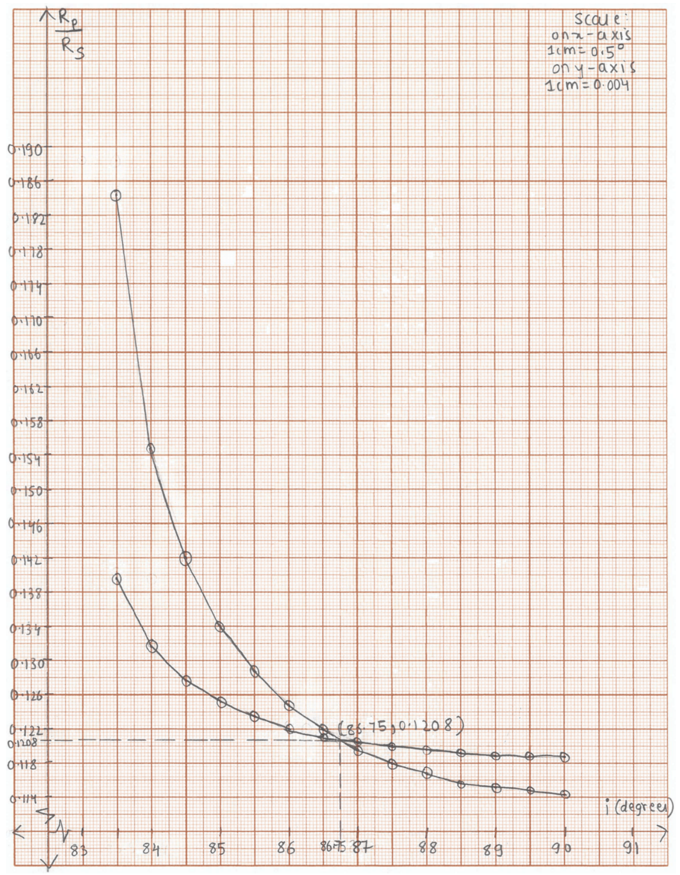
However, it is enough to plot around the point of intersection (can be deduced from the table above), to get a better resolution for the coordinates of the intersection point.

(D01.7d) Solution:

Intersection point of the graphs of $(R_p/R_s)$ vs $i$ for $\lambda_B$ and $\lambda_R$ will give the values of both quantities.

Values deduced from either graph:

\left(\frac{R_p}{R_s}\right)=0.1208

\Longrightarrow\quad R_p=0.1208\times1.2R_\odot

\boxed{R_p=0.145R_\odot}

and

\boxed{i=86.75^\circ}

(D01.8) Solution:

Estimated mass of the planet P $M_p=6.93\times10^{-4}M_\odot=1.389\times10^{27}\ \mathrm{kg}$

Estimated radius of the planet P $R_p=0.145R_\odot=1.009\times10^8\ \mathrm m$

$\therefore$ Average density of the planet $=320\ \mathrm{kg\,m^{-3}}$

The average density of the planet P is much less than that of Jupiter (a known gaseous planet). Hence the planet P is GASEOUS.

D02 Summary Answersheet — SA-1

Summary Answersheet — FRONT

Contestant Code: ______ – ______

Q. No. D02 · Page No. SA-1

Final answers

(D02.1a) Marks (3.0)

CME Name	$u$ ( $\mathrm{km\,s^{-1}}$ )	$v$ ( $\mathrm{km\,s^{-1}}$ )	$\tau$ (h)
CME-A	804	470	74.5
CME-B	247	360	127.5
CME-C	523	396	103.5
CME-D	830	415	71.0
CME-E	665	400	104.5
CME-F	347	350	101.5
CME-G	446	375	99.5
CME-H	155	360	97.0
CME-I	1016	515	67.0
CME-J	683	410	54.0

(D02.1b) Marks (15.0)

Graph number: D02.1b

$m=$ ______

$\alpha=$ ______

D02 Summary Answersheet — SA-2

Summary Answersheet — BACK

Contestant Code: ______ – ______

Q. No. D02 · Page No. SA-2

Final answers

(D02.1c) Marks (4.0)

CME Name	$a_{\mathrm{model}}$ ( $\mathrm{m\,s^{-2}}$ )
CME-A
CME-B
CME-C
CME-D
CME-E
CME-F
CME-G
CME-H
CME-I
CME-J

$\delta a_{\mathrm{rms}}=$ ______

(D02.2a) Marks (4.0)

$\tau_{1,\mathrm m}=$ ______ h

$\tau_{2,\mathrm m}=$ ______ h

(D02.2b) Marks (2.0)

	VALID	NOT VALID
CME-1
CME-2

D02 Summary Answersheet — SA-3

Summary Answersheet — FRONT

Contestant Code: ______ – ______

Q. No. D02 · Page No. SA-3

Final answers

(D02.3a) Marks (6.0)

C1:

$\delta R_D=$ ______ $R_\odot$

C2:

$\delta R_D=$ ______ $R_\odot$

(D02.3b) Marks (4.0)

Data Point	$t$ (h)	C3: $R_D(t)$ ( $R_\odot$ )	C4: $R_D(t)$ ( $R_\odot$ )
P5	21.0
P6	50.0
P7	85.0
P8	111

(D02.3c) Marks (10.0)

Graph number: D02.3c

D02 Summary Answersheet — SA-4

Summary Answersheet — BACK

Contestant Code: ______ – ______

Q. No. D02 · Page No. SA-4

Final answers

(D02.3d) Marks (4.0)

C3: $|\delta\tau|=$ ______

C4: $|\delta\tau|=$ ______

(D02.3e) Marks (1.0)

TRUE □ FALSE □

(D02.4) Marks (7.0)

CME Name	$u$ ( $\mathrm{km\,s^{-1}}$ )	$v$ ( $\mathrm{km\,s^{-1}}$ )	$\tau$ (h)
CME-A	804	470	74.5
CME-B	247	360	127.5
CME-C	523	396	103.5
CME-D	830	415	71.0
CME-E	665	400	104.5
CME-F	347	350	101.5
CME-G	446	375	99.5
CME-H	155	360	97.0
CME-I	1016	515	67.0
CME-J	683	410	54.0

$V_{s,\mathrm{avg}}=$ ______

Total: ______

End of Summary Answersheet

Оригинал в Архива: Data-Analysis-Questions.pdf · официални решения: Data-Analysis-Solutions.pdf · допълнителни данни: Data-Analysis-Summary-Answersheet.pdf